STrenD: Subspace Trend Discovery
| (49 intermediate revisions by one user not shown) | |||
| Line 1: | Line 1: | ||
| − | == | + | == Description == |
| − | + | The goal of this project is to develop unsupervised algorithms for discovering previously unknown subspace trends in high-dimensional data sets without the benefit of prior information. A subspace trend is a sustained pattern of gradual/progressive changes within an unknown subset of feature dimensions. A fundamental challenge to subspace trend discovery is the presence of irrelevant data dimensions, noise, outliers, and confusion from multiple subspace trends driven by independent factors that are mixed in with each other. These factors can obscure the trends in traditional dimension reduction and projection based data visualizations. We aim to efficiently select trend-relevant features and derive meaningful 2-D or 3-D visualizations. The proposed algorithm is broadly applicable to exploratory analysis of high-dimensional data including visualization, hypothesis generation, knowledge discovery, and prediction in diverse other applications. | |
| − | + | Please find more details in the following paper: | |
| − | + | http://ieeexplore.ieee.org/xpl/articleDetails.jsp?arnumber=7015603 | |
| − | + | == Software Interface == | |
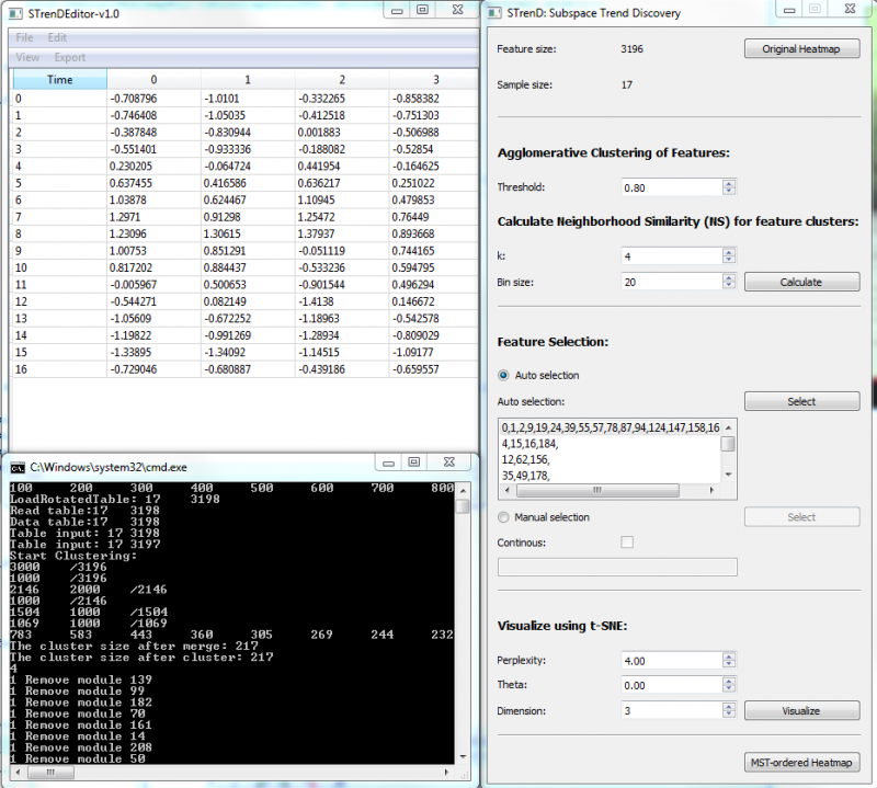
| − | + | [[File:STrendInterface.png|800px |thumb|center| '''Fig. 1''' Software interface]] | |
| − | + | 1. Load Tab-delimited txt file. If columns are features and rows are samples, '''File/Load Table'''; If columns are samples and rows are features, '''File/Load Rotated Table'''; | |
| − | + | 2. '''Calculate''' for feature clustering and pair-wise neighborhood similarity (NS); | |
| − | + | ||
| − | + | 3. '''Auto selection''': push '''select''' for automatic thresholding on NS matrix to provide a list of non-overlapping feature subsets (size >=3). The largest subset, on top of the list, is selected by default; | |
| − | + | ||
| − | + | 4. '''Manual selection''': push '''select''' to visualize co-clustered NS matrix and select a group of features that have high NS values by left clicking on the top-left starting square and releasing on the right-bottom ending square. The user can also input feature cluster index in the editor, separated by comma; The old selection is kept when '''Continuous''' is checked, or else the old selection is erased. | |
| − | + | ||
| − | ''' | + | 5. '''Visualize''' to provide a 2-D or 3-D visualization using t-SNE("dimension" higher than 3 would be visualized in 2D with a selected pair of dimensions); |
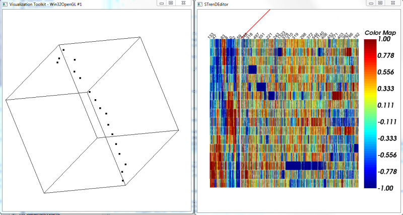
| − | + | 6. '''MST-ordered Heatmap''' to visualize a heatmap with rows arranged by the depth-first order of MST on selected data and columns arranged by a hierarchical clustering of features. The selected ones are separated by a red line from the rest. | |
| − | |||
| − | |||
| − | == | + | == Download == |
| − | + | ||
| + | STrenD-v1.0 (implemented in C++) is available to download at | ||
| + | |||
| + | '''Windows 64 bit''': | ||
| + | |||
| + | '''Release''': | ||
| + | https://github.com/YanXuHappygela/STrenD-release-1.0 | ||
| + | |||
| + | '''Source codes''': | ||
| + | https://github.com/YanXuHappygela/STrenD-source-1.0 | ||
| + | |||
| + | Matlab wrapper is coming up soon! | ||
| + | |||
| + | If you have any problem with the software, please report to ''yansoftwareus@gmail.com''. Thank you. | ||
| + | |||
| + | == Test on Cell Cycle Microarray data == | ||
| + | |||
| + | |||
| + | For test dataset "cellCycleMicroarray.txt" with default param settings: | ||
| + | |||
| + | '''File/Load Rotated Table''' (cellCycleMicroarray.txt) -> '''Auto selection''':'''select''' ->'''Visualize'''->'''MST-ordered Heatmap''' | ||
| + | |||
| + | === Actively-linked Visualization === | ||
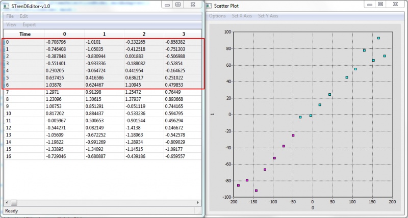
| + | [[File:STrend2DProj.jpg |800px |thumb|center| '''Fig. 2''' 2D projection of the data with selected features. Selection in the table and 2D scatter plot are synchronized.]] | ||
| + | |||
| + | |||
| + | [[File:STrenDTestRs1.png|800px |thumb|center| '''Fig. 3''' 3D projection of the data with selected features and the MST-ordered Heatmap. ]] | ||
| + | |||
| + | === Output Files === | ||
| + | |||
| + | For test dataset "cellCycleMicroarray.txt" with 17 samples of 3196 dimensions, clustering sigma = 0.8, k = 4: | ||
| + | |||
| + | 1. '''3196_17_0.8_clustering.txt''': agglomerative clustering result, containing index and feature names; | ||
| + | |||
| + | 2. '''3196_17_0.8_4_NS.txt''': pair-wise neighborhood similarity matrix of feature clusters; | ||
| + | |||
| + | 3. '''Shanbhag.txt''': intermediate outputs for Shanbhag thresholding; | ||
| + | |||
| + | 4. '''3196_17_0.8_4_AutoSelFeatures.txt''': selected feature index and names; | ||
| + | |||
| + | 5. '''data_selected_vis.txt''': table of normalized data with selected features for visualization; | ||
| + | |||
| + | 6. '''vis_coordinates.txt''': output coordinates for visualization after dimension reduction by t-SNE. | ||
Latest revision as of 15:13, 24 February 2015
Contents |
Description
The goal of this project is to develop unsupervised algorithms for discovering previously unknown subspace trends in high-dimensional data sets without the benefit of prior information. A subspace trend is a sustained pattern of gradual/progressive changes within an unknown subset of feature dimensions. A fundamental challenge to subspace trend discovery is the presence of irrelevant data dimensions, noise, outliers, and confusion from multiple subspace trends driven by independent factors that are mixed in with each other. These factors can obscure the trends in traditional dimension reduction and projection based data visualizations. We aim to efficiently select trend-relevant features and derive meaningful 2-D or 3-D visualizations. The proposed algorithm is broadly applicable to exploratory analysis of high-dimensional data including visualization, hypothesis generation, knowledge discovery, and prediction in diverse other applications.
Please find more details in the following paper: http://ieeexplore.ieee.org/xpl/articleDetails.jsp?arnumber=7015603
Software Interface
1. Load Tab-delimited txt file. If columns are features and rows are samples, File/Load Table; If columns are samples and rows are features, File/Load Rotated Table;
2. Calculate for feature clustering and pair-wise neighborhood similarity (NS);
3. Auto selection: push select for automatic thresholding on NS matrix to provide a list of non-overlapping feature subsets (size >=3). The largest subset, on top of the list, is selected by default;
4. Manual selection: push select to visualize co-clustered NS matrix and select a group of features that have high NS values by left clicking on the top-left starting square and releasing on the right-bottom ending square. The user can also input feature cluster index in the editor, separated by comma; The old selection is kept when Continuous is checked, or else the old selection is erased.
5. Visualize to provide a 2-D or 3-D visualization using t-SNE("dimension" higher than 3 would be visualized in 2D with a selected pair of dimensions);
6. MST-ordered Heatmap to visualize a heatmap with rows arranged by the depth-first order of MST on selected data and columns arranged by a hierarchical clustering of features. The selected ones are separated by a red line from the rest.
Download
STrenD-v1.0 (implemented in C++) is available to download at
Windows 64 bit:
Release: https://github.com/YanXuHappygela/STrenD-release-1.0
Source codes: https://github.com/YanXuHappygela/STrenD-source-1.0
Matlab wrapper is coming up soon!
If you have any problem with the software, please report to yansoftwareus@gmail.com. Thank you.
Test on Cell Cycle Microarray data
For test dataset "cellCycleMicroarray.txt" with default param settings:
File/Load Rotated Table (cellCycleMicroarray.txt) -> Auto selection:select ->Visualize->MST-ordered Heatmap
Actively-linked Visualization
Output Files
For test dataset "cellCycleMicroarray.txt" with 17 samples of 3196 dimensions, clustering sigma = 0.8, k = 4:
1. 3196_17_0.8_clustering.txt: agglomerative clustering result, containing index and feature names;
2. 3196_17_0.8_4_NS.txt: pair-wise neighborhood similarity matrix of feature clusters;
3. Shanbhag.txt: intermediate outputs for Shanbhag thresholding;
4. 3196_17_0.8_4_AutoSelFeatures.txt: selected feature index and names;
5. data_selected_vis.txt: table of normalized data with selected features for visualization;
6. vis_coordinates.txt: output coordinates for visualization after dimension reduction by t-SNE.


