Harmonic Co-clustering Heatmap
(→Heatmap) |
(→Coupled Geometry) |
||
| (8 intermediate revisions by one user not shown) | |||
| Line 8: | Line 8: | ||
== Coupled Geometry == | == Coupled Geometry == | ||
| − | For a given data matrix, there are two spaces that we consider, the row space and the column space. A coupled geometry of the two spaces is derived by taking the tensor product of the hierarchical partition tree from each space. Again we use the concept of basis function for the coupled geometry, folders become rectangular in the tensor space. The basis function in the tensor space is simply the tensor product of the basis function induce by each local geometry.Schematic illustration as shown | + | For a given data matrix, there are two spaces that we consider, the row space and the column space. A coupled geometry of the two spaces is derived by taking the tensor product of the hierarchical partition tree from each space. Again we use the concept of basis function for the coupled geometry, folders become rectangular in the tensor space. The basis function in the tensor space is simply the tensor product of the basis function induce by each local geometry.Schematic illustration as shown: |
[[Image:p2.png|150px|center|thumb|rectangular basis]] | [[Image:p2.png|150px|center|thumb|rectangular basis]] | ||
== Smoothness == | == Smoothness == | ||
As is known in the domain of harmonic analysis, signal or dataset is smooth with respect to low coefficients entropy. We compute the first order norm entropy of the expansion based on orthogonal basis function induced from the global coupled geometry in each iteration until it reaches the threshold that we set. | As is known in the domain of harmonic analysis, signal or dataset is smooth with respect to low coefficients entropy. We compute the first order norm entropy of the expansion based on orthogonal basis function induced from the global coupled geometry in each iteration until it reaches the threshold that we set. | ||
| + | |||
| + | == Algorithm== | ||
| + | The algorithm is shown in the flow chart below: | ||
| + | [[Image:al.png|400px|center]] | ||
== Heatmap == | == Heatmap == | ||
Given a data matrix, it is easy to visualize it in a heatmap. Pictures below show a heatmap of raw data matrix and a heatmap after applying the harmonic co-clustering algorithm. | Given a data matrix, it is easy to visualize it in a heatmap. Pictures below show a heatmap of raw data matrix and a heatmap after applying the harmonic co-clustering algorithm. | ||
| − | [[Image:rawh.png| | + | <center>[[Image:rawh.png|400px|Raw Data Heatmap]] [[Image:reh.png|400px|Processed Data Heatmap]]</center> |
| − | [[Image:reh.png| | + | |
| − | + | ||
| − | + | ||
| − | + | ||
| − | + | ||
| − | + | ||
| − | + | ||
Latest revision as of 23:36, 15 November 2012
Contents |
Introduction
Co-clustering is a data mining technique that clusters both rows and columns of a data matrix simultaneously. It looks for clusters of similar objects and correlated features that distinguish groups of objects. Harmonic co-clustering is a co-clustering method that achieves clusters in both row space and column space, block structures of a data matrix based on discrete harmonic analysis. Harmonic basis are induced from a constructed coupled geometry of the two spaces. We obtain the coupled geometry by taking the tensor product of local geometry which is captured by a hierarchical partition tree in both row space and column space. Data set is smooth and block structure is obtained with respect to low entropy of expansion coefficients on data matrix. The algorithm proceeds in an iterative way that each local geometry is constructed on the update version of geometry of the other space. By iteratively doing this, the data set become more and more compact and smooth each time. The entropy of expansion coefficients will converge to a low value as thresholdded.
Hierarchical Partition Tree
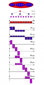
The geometrical structure of a high dimensional data cloud is assumed to be captured by a finer and finer hierarchical partition tree in different levels. Different levels represent different resolutions of the dataset. The bottom level of the tree is comprised with N (number of points) folders each consists a single member from N elements. The top level of the hierarchical tree is comprised with one folder which is the combination of all elements. In the middle levels, folders are combinations of elements from lower levels. All those folders are obtained by applying a simple heuristic k-means clustering on lower level data points. Each folder is denoted as a new data point by a linear combination of the all elements that make up the folder. Each level of the partition tree is a representation of the data cloud, and each level span a subspace of the could. The bottom level which includes each single elements spans the whole data space. Since the higher level is linear combination of the lower level, the space it spans is a subspace, thus there exist an orthogonal subspace which can together comprise the space spanned by lower level. Those basis element exists in the orthogonal subspace is supported by the folders we have. A briefly schematic illustration of the concept is as shown in the figure on the right.
Coupled Geometry
For a given data matrix, there are two spaces that we consider, the row space and the column space. A coupled geometry of the two spaces is derived by taking the tensor product of the hierarchical partition tree from each space. Again we use the concept of basis function for the coupled geometry, folders become rectangular in the tensor space. The basis function in the tensor space is simply the tensor product of the basis function induce by each local geometry.Schematic illustration as shown:
Smoothness
As is known in the domain of harmonic analysis, signal or dataset is smooth with respect to low coefficients entropy. We compute the first order norm entropy of the expansion based on orthogonal basis function induced from the global coupled geometry in each iteration until it reaches the threshold that we set.
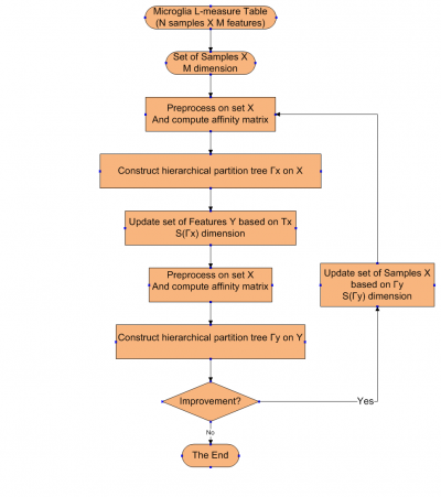
Algorithm
The algorithm is shown in the flow chart below:
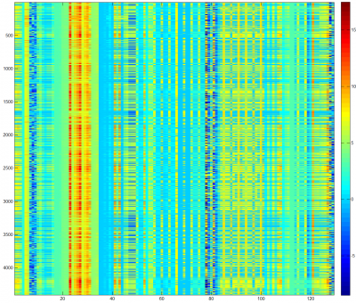
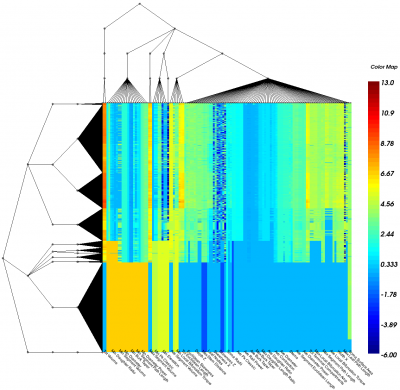
Heatmap
Given a data matrix, it is easy to visualize it in a heatmap. Pictures below show a heatmap of raw data matrix and a heatmap after applying the harmonic co-clustering algorithm.


