Features Events
Contents |
Worm Features and Events
In our system, after tracking the results are fed to the Features and Events module for quantitative analysis. Our automated system quantitates features describing the worm shape(morphology,posture), motion(movement, bending or waving), and events(reversal,omega bend or foraging), etc. Most features are collected from the literature([2-10]) or requested by the Biologists, others are based on our old features [1].
Features and Events List
All the features and events measured by the automated system are listed below. Details about the computation of some features can be found in next section.

Algorithms and Examples
Track and SktAgl Feature Sets
Both feature sets are based on the skeleton curve after rotation(so the resulting skewer line (line passing through centroid and parallel to the line liking head and tail) becomes the x-axis) and offset(so the resulting centroid becomes the origin), as shown in Figure 1.
- Track Features:
- Track.Amp,Track.Length, Track.Elongation Factor and Track.Compactness are easy to compute given the information on Figure.1.
- To calculate Track.WaveLength, we treat the rotated skeleton points as sinusodial wave as in [8]. We first interpolate in x coordinates of the same interval, then perform Fast Fourier Transform. The frequency component with maximum magnitude is selected, interval between two x consecutive coordinates times the inverse of this frequency represents the wavelength of the sinusodial wave.
- SktAgl Features:
- SktAlg.Avg is the average of the angles between the x-axis and the line linking the skeleton points and the centroid after rotate and offset the skeleton points (Figure 1). [8] suggests that this feature helps in identifying omega turns, since the skeleton point set of an worm in an omega turn has a smaller Track.Elongation value and larger Track.Amp and SktAgl.Ave values.
- SktAlg.Max is the max angle between skeleton points and centroid.
Figure.2 shows an example for the two feature sets.


Symmetry and Curvature Feature Sets
Figure.3 shows the information used for calculating Symmetry and Curvature feature sets:(1)Centroid (2)Head Point (3)Tail Point (4)θi :Angle between ployline segments of the skeleton curve (5)Distance from each point to the line connecting head and tail.
- Symmetry Features: [4] designed three features to measures the similarity of worm central line with a perfect sine wave.
- Symmetry.Amp is the sum of the absolute distance from points on the skeleton to the line connecting head and tail.
- Symmetry.SignedDist is the sum of the signed distance from points to the line. Smaller value of this feature suggests larger symmetry against the line.
- HCTAngle is the angle between the line from centroid to head, and the line from centroid to tail.
- Curvature Features: Curvature is used to express the worm conformation.
- Curvature.Avg is the average of the signed curvature value:
 , where θi is the angle between ployline segments of the skeleton curve, L is the length of the segments and N is the number of skeleton points.
- Curvature.Amp is the average of the unsigned curvature value:
 . This feature is used for describing coil degree in [1]. Skeleton curve of a worm in an omega turn or coiling worm usually has a higher Curvature.Amp value. Curvature as a function of position along the skeleton and time (
 ) also can be used for computing the bending frequency(see below the datail algorithm)
- Curvature.Avg is the average of the signed curvature value:


Source and Waving Feature Sets
- Source Features: this feature set uses information from Figure.5 to describe the posture and movement of worm relative to the pheromone source. Source.Bearing, Source.HeadDirection and Source.Translation describe bearing, head direction and worm translation relative to the pheromone source respectively.
- Waving Features: two features, BodyWaving.Pushing and BodyWaving.HdTRatio are used in [8] to express the waving of the worm body.
- BodyWaving.Pusing: Skeleton point sets in time τ and τ + 1 are first superimposed to have a common centroid, which allows the calculation of invidual movement of skeleton points regardless of the whole body movement. Then BodyWaving.Pusing is obtained by computing the ratio of the mean distance all skeleton points traveled between time τ and τ + 1 to the actual distance traveled by the worm’s centroid during the same time interval.
- BodyWaving.HdTRatio: The ratio of head movement distance to tail movement distance during a time interval τ to τ + 1 [8][9].


Other Features
- Bending Frequency: following the algorithm in [6], worm bending frequency is calculated based on the curvature function κ(i,t), as shown in Figure.7. Let
![K_i(w)=\vert{F[\kappa(i,t)]}\vert](/mw/images/math/a/2/c/a2c86d7749d780b2e6815feea9072030.png) denote the magnitude of the Fourier transform at the ith location along the worm body, and
denote the magnitude of the Fourier transform at the ith location along the worm body, and  denote the frequency maximizing the magnitude response at the ith location, the bending frequency can be expressed as:
 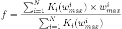 , which is the weighted average frequency over the worm body.


References
- [1] Nicolas Roussel, A Computational Model for C.elegans locomotory behavior: Application to Multi-Worm tracking. Phd Thesis 2007.
- [2] Christopher J Cronin, An automated system for measuring parameters of nematode sinusoidal movement. BMC Genet 2005.
- [3] Huang KM, Cosman P, Schafer WR, Machine vision based detection of omega bends and reversals in C. elegans. Journal of Neuroscience Methods, Vol. 158, Issue 2, pp. 323-336, December 2006.
- [4] Wei Geng, Pamela Cosman, Automatic Tracking, Feature Extraction and Classification of C. elegans Phenotypes. IEEE Transactions on Biomedical Engineering, Vol. 51, No. 10, pp. 1811--1820, October 2004.
- [5] Huang KM, Cosman P, Schafer WR, Automated detection and analysis of foraging behavior in Caenorhabditis elegans. Journal of Neuroscience Methods,2008.
- [6]Ebraheem Fontaine, Automated visual tracking for studying the ontogeny of zebrafish swimming. Journal of Experimental Biology, 2008.
- [7] W.H. Wang, Y. Sun, A Micropositioning System with Real-Time Feature Extraction Capability for Quantifying C. elegans *Locomotive Behavior. IEEE International Conference on Automation Science and Engineering, 2007. CASE 2007.
- [8] Zhaoyang Feng, Quantitative analysis of C. elegans: Algorithms to calculate behavioral and morphological features. BMC Bioinformatics 2004.
- [9] Zhaoyang Feng, An imaging system for standardized quantitative analysis of C.elegans behavior. BMC Bioinformatics 2004.
- [10] Jesse M. Gray, Joseph J. Hill, A circuit for navigation in Caenorhabditis elegans. PNAS 2005.