FARSIGHT Tutorials/5-Label
Contents |
Details
- Goal: This tutorial is intended to show you how to use the specialized FARSIGHT segmentation modules to process a 4-dimensional (5-Label) image from start to finish.
- Duration: 1 hour
- Requisites: Basic familiarity with Python commands
- Materials: FARSIGHT Installed
Basic Concepts
Farsight uses the "divide and conquer" approach. Each of the channels (labels) in the images is processed individually and the results combined at the end to create a complete solution. Each "module" in farsight is a stand-alone application that can be executed from within python. Python is used to allow for easy parameter adjustment and pipelining of segmentation modules. Most modules require two inputs - 1. Parameter File (XML), 2. Image File.
Starting the Interpreter
The first thing you need to do is to start your Python interpreter
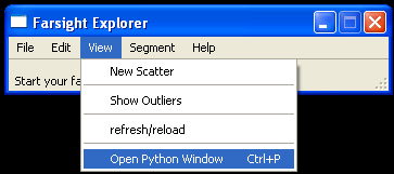
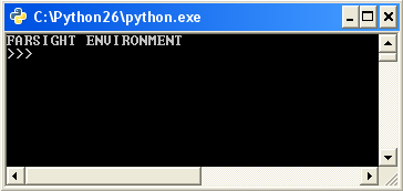
- From the Farsight GUI select View > Open Python Window to start the python interpreter.
Reading an image from a file and Showing it
Getting example image
The example image is available at: link not available
This image was acquired using the spectral fingerprinting software available on the Zeiss META system, 32-point spectral fingerprints were captured for each fluorophore, and the built-in linear unmixing software was used to isolate the signals into a set of five individual channels labeling: (i) cell nuclei (CyQuant); (ii) astrocytes (GFAP); (iii) neurons (Nissl); (iv) blood vessels (EBA); and (v) microglia (Iba1). The original 5-Label Image has the Ziess .LSM extension. For the purposes of this tutorial we have split the image into its 5 channels and cropped a small region from each.
Showing an image
The sample image can be viewed from the Farsight GUI using the File|Load Image command.
Part II: Processing the image
Note that the steps below are specific to windows machine with (.exe) files - but the scripts can be modified easily for other platforms.
Nuclear Segmentation
The first step in nuclear segmentation is creating the parameter file. The details of how to choose these parameters can be found on the Nuclear Segmentation page. Below we provide default parameters that will work well for the sample image provided.
 high_sensitivity	   :	1
 LoG_size	           :	30
 min_scale	           :	2
 max_scale	           :	7
 xy_clustering_res	   :	2
 z_clustering_res	   :	1
 finalize_segmentation	   :	0
 sampling_ratio_XY_to_Z   :	5
 Use_Distance_Map	   :	1
 refinement_range	   :	3
Save this file as NucParams.ini
Make sure that your current Python working directory is set to the location of the input file using this command:
 import os
 os.getcwd()
You can change the working directory with this command:
os.chdir(dirname)
Now you are ready to trigger the segmentation module:
 import subprocess
 subprocess.call(['segment_nuclei.exe', 'NM_crop1_Nuc.pic', 'NM_crop1_Nuc_label.pic', 'NucParams.ini'])
The command should execute the nuclear segmentation on the image named NM_crop1_Nuc.pic using the parameters in NucParams.ini and save the output as NM_crop1_Nuc_label.pic. The output will be a multi-page label map image - an image the same size as the input image with each pixel being assigned a label (zero for background)
Vessel Segmentation
At present the vessel segmentation module will use decent default parameters and requires no input parameter file. Details of the module can be found on the Vessel Laminae Segmentation page. To execute the vessel segmentation module us this python command:
subprocess.call(['vessel_segmentation.exe', 'NM_crop1_EBA.pic', 'NM_crop1_EBA_surface.pic'])
Be patient - this step will take several minutes. The output is a binary image named NM_crop1_EBA_surface.pic
Trace Astrocytes
The tracing module requires a single XML file as input. This XML file must specify the tracing parameters and the input image name. Create an xml file called NM_crop1_GFAP_TracingParams.xml with the following content:
 <parameters>
   <parameter name="input_image" value="NM_crop1_GFAP.pic"/>
   <parameter name="SeedsSamplingDensity" value="5"/>
   <parameter name="MinTemplateLength" value="4"/>
   <parameter name="MaxTemplateLength" value="12"/>
   <parameter name="MinShiftDistance" value="2"/>
   <parameter name="MaxShiftDistance" value="10"/>
   <parameter name="DirectionFreedom" value="8"/>
   <parameter name="StepSize" value="2"/>
   <parameter name="TracingSensitivity" value="5"/>
   <parameter name="MaxAllowedStoppingViolations" value="3"/>
   <parameter name="RelativeShiftDistance" value="2"/>
   <parameter name="DetectSoma" value="n"/>
   <parameter name="MergeTraceEndPoints" value="n"/>
   <parameter name="DetectBranchPoints" value="y"/>
   <parameter name="MaxBranchSearchDistance" value="10"/>
 </parameters>
Now trigger the tracing module:
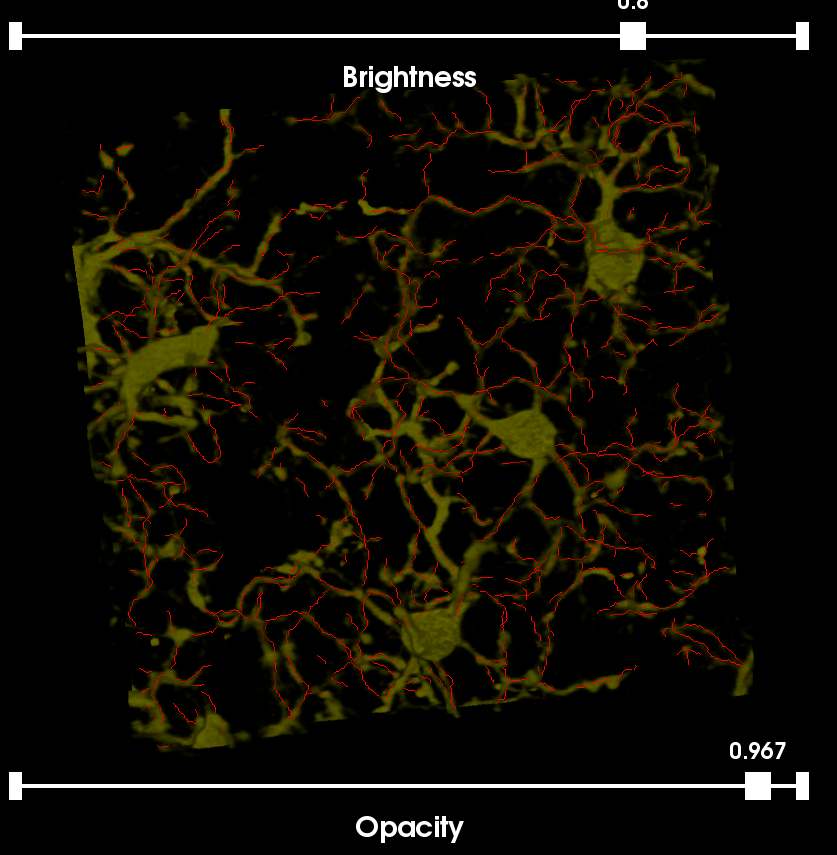
subprocess.call(["RPITrace3D.exe", 'NM_crop1_GFAP_TracingParams.xml'])
The output will be a TracedPoints.xml file in the RPI Tracing File format.
Trace Microglia
The microglia can be traced exact same way as the astrocytes. Simply create a new parameter file 'NM_crop1_Iba1_TracingParams.xml' and change the "input_image" parameter to "NM_crop1_iba1.pic"
<parameter name="input_image" value="NM_crop1_Iba1.pic"/>
Then trace microglia:
subprocess.call(["RPITrace3D.exe", 'NM_crop1_Iba1_TracingParams.xml'])
Compute Associative Features
Once these 4 channels have been segmented (Nuclei, Blood Vessels, Astrocytes, and Microglia) we can compute the associated features. These features will be used for classifying nuclei as belonging to one of the 4 cell types. The fifth channel in the image (Nissl) is used for classifying neurons.
Create an association definition file and save it as NM_crop1_AssocDefs.xml:
 <ObjectAssociationRules SegmentationSource="NM_crop1_Nuc_label.tiff" NumberOfAssociativeMeasures="5">
 <AssociationRule Name="Nissl_sig" Target_Image="NM_crop1_Nissl.pic" Outside_Distance="5" Inside_Distance="0" Use_Whole_Object="False" Association_Type="TOTAL" />
 <AssociationRule Name="Iba1_sig" Target_Image="NM_crop1_Iba1.pic" Outside_Distance="0" Inside_Distance="0" Use_Whole_Object="True" Association_Type="AVERAGE" />
 <AssociationRule Name="GFAP_sig" Target_Image="NM_crop1_GFAP.pic" Outside_Distance="5" Inside_Distance="0" Use_Whole_Object="False" Association_Type="AVERAGE" />
 <AssociationRule Name="EBA_sig" Target_Image="NM_crop1_EBA_surface.pic" Outside_Distance="5" Inside_Distance="0" Use_Whole_Object="False" Association_Type="TOTAL" />
 <AssociationRule Name="Dist_to_Bldv" Target_Image="NM_crop1_EBA_surface_distance_map.tif" Outside_Distance="0" Inside_Distance="0" Use_Whole_Object="True"
   Association_Type="AVERAGE"/>
 </ObjectAssociationRules>
Make sure that the image names in this file match images that exist in the current directory. The surface_distance_map file should be created by the vessel segmentation module already.
subprocess.call(['compute_associative_measures.exe', 'NM_crop1_AssocDefs.xml'])
Compute Intrinsic Features
We can also compute intrinsic features for each nucleus. These features will provide useful information for classification and editing of objects. This function will produce an XML file that can be opened in the Farsight GUI using the File > Load Result command. The features and file are specific to the nuclear channel (all features are linked to a single nucleus)
subprocess.call(['compute_nuclei_features.exe', os.getcwd(), 'NM_crop1_Nuc.pic', 'NM_crop1_Nuc_label.pic, 'NM_crop1_AssocDefs_AssocFeatures.XML'])
For more information about the types of features that are calculated for blobs please see the Intrinsic Features of Blobs page.
Classification
Classification is a work in progress. Results can be viewed without this step.
Visualization/Editing
Traces
To edit microglia or astrocytes using Trace Editor:
subprocess.call(['trace_editor.exe', NM_crop1_Iba1TracedPoints.xml', 'NM_crop1_Iba1.pic'])
or
subprocess.call(['trace_editor.exe', NM_crop1_GFAPTracedPoints.xml', 'NM_crop1_GFAP.pic'])
Blobs
To edit nuclei use the Farsight GUI: File > Load Result
- Select the .xml file that was generated by the compute_nuclei_features program
- This should open 3 new windows:
3D Rendering
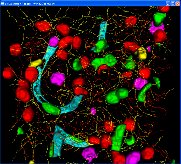
A complete 3D rendering of the results can be created using the render module. This module requires a single input file:
 1 1 3.5
 NM_crop1_EBA_surface.pic 0 1 1
 NM_crop1_GFAPTracedPoints.xml 1 0 0
 NM_crop1_Iba1TracedPoints.xml 1 1 0
 NM_crop1_Nuc.pic 1 0 0
The first line specifics the image spacing (x y z). Then provide each result file that should be rendered followed by the RGB components to use to color that image. The rendering will take a little time so be patient. Save the file as NM_crop1_render.txt The rendering module is called like this:
subprocess.call(['render.exe', 'NM_crop1_render.txt'])


