Trace Editor/Features
From FarsightWiki
(Difference between revisions)
(→Feature List) |
m (→Algorithms) |
||
| Line 78: | Line 78: | ||
Method: Larger gaps need new segments created, <br />new Trace Bits must be added, <br />smoothing operator. | Method: Larger gaps need new segments created, <br />new Trace Bits must be added, <br />smoothing operator. | ||
| − | [[Image:MergingBranching.gif|800px|thumb|right|Example showing how Merging and branching are interconnected. The Merging that creates sharp turns needs to be smoothed. The Traces need to create a new branch point and trace bits to interpolate the original ]] | + | [[Image:MergingBranching.gif|800px|thumb|right|Example showing how Merging and branching are interconnected. The Merging that creates sharp turns needs to be smoothed. The Traces need to create a new branch point and trace bits to interpolate the original path of the branch. ]] |
*Curve fitting to find trend of: | *Curve fitting to find trend of: | ||
| Line 87: | Line 87: | ||
**Most probable vector | **Most probable vector | ||
**Avoid creating edges | **Avoid creating edges | ||
| − | |||
3: '''Branch Points''' | 3: '''Branch Points''' | ||
Revision as of 15:38, 2 July 2009
Feature computation for Trace Editor
Feature List
| Feature | Description | Equation or Variable |
|---|---|---|
| Gap Size | Minimum distance between endpoints of two traces | 
|
| Angle | The angle created between two traces normalized as vectors | 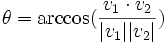
|
| Path Length | Total length along a trace, indicated by the size of the trace | 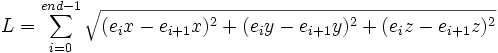
|
| Euclidean Distance | Straight line distance between the endpoints of a trace | 
|
| Fragmentation Smoothness | Ratio of Path Length to Euclidean Distance[1] | 
|
| Maximum Gap Distance | The maximum distance between endpoints that can be merged | Δ |
| Weights | The weights are used in the cost algorithm | α β |
| Cost | Weighted scalar evaluating the merge | 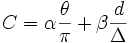
|
| Curvature | The Hessian matrix for checking branching point existence and interpolating the path. (Still under consideration) | ![\left[\begin{array}{ccc}
f(x)_{xx}(X) + \frac{\alpha}{2}f_{yy}(X) + \frac{\alpha}{2}f_{zz}(X) & (1-\alpha)f_{xy}(X) & (1-\alpha)f_{xz}(X) \\
(1-\alpha)f_{xy}(X) & f_{yy}(X) + \frac{\alpha}{2}f(x)_{xx}(X) +\frac{\alpha}{2}f_{zz}(X) & (1-\alpha)f_{yz}(X) \\
(1-\alpha)f_{xz}(X) & (1-\alpha)f_{yz}(X) & f_{zz}(X) + \frac{\alpha}{2}f(x)_{xx}(X) +\frac{\alpha}{2}f_{yy}(X)
\end{array} \right]](/mw/images/math/8/6/2/86265c277f698370dbb9b8bbf95c9619.png)
|
| Parent | Considering nerves branching from the soma are a tree like structure, a parent point can be used to find a cycle. |
Algorithms
The algorithms suggested are used to control the editing process allowing for rule based cluster editing. The Goal is to complete group editing in five steps.

1: Merge Small Gaps
Goal: Create longest continuous trace segments by merging close endpoints
Methods: Nearest neighbors  (Closest end points),
Rejection based on conflicts and thresholds
- Minimal distance between end points
- Angle between traces- The angle is measured between the two traces by computing the norm of their vectors and the dot product.
The equation is: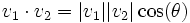 which when solved for θ is:
- Path length- If the end points are not the best fit for the merge this is when path length is considered. An example of this would be a peak in the neurite on completion the given merge. An example if given in an image in this section. This is also discussed in large gaps being that in the large gap case these type of error cause more of a problem. a sharp change in a neurite in a subsection prior to the end point would indicate this error. Merging at the sharp direction change( especially in the small gap case) can alleviate the neurite of peaks.
- Gap distance is too large- If the distance between the two points e1, e2 is greater then the excepted distance for a small gap then they will not be considered. This is tested prior to computing the angular difference due to the expense of computing angles. Between this case and the angular case we have a similar metric to the cost function in "Automated Three-Dimensional Tracing of Neurons in Confocal and Brightfield Images"; however, the conditions under which we check for small gaps is when there are only two end points to be merged
- Consider possibility of loops Even though this might not be possible in the 3D case, if we were to use a 2D projection of the picture there might be a situation where multiple breaks might end in a loop. consider the cross sectioning of two neurites. A gap at anyone of the intersections could cause connection problems. This matter on the cost function this could mean a loop will form. This formation might not be correct, but I think we should at least consider it.
- Angle between traces- The angle is measured between the two traces by computing the norm of their vectors and the dot product.

- Another trace is a better fit (Cost Function)
- Smallest gap
- Better Angular alignment
- "Bad merge"
- The merge causes corners
- Needs to be smoothed
2: Interpolate Large Gaps
Goal: Connect Large gaps that step 1 cannot  simply connect by addition of a  single cell
Method: Larger gaps need new segments created,
new Trace Bits must be added,
smoothing operator.

- Curve fitting to find trend of:
- Direction
- Curvature
- Interpolation
- Extend the line
- Most probable vector
- Avoid creating edges
3: Branch Points
Goal: Detect and control Branching
Method: Detect most probable intercepts,
Determination of main branch and child,
Type of branch point
- Distance maps
- Nearest neighbors (traces)
- Closest trace bits
- Angle of intercept
- Interpolation
4: Soma Detection
Goal: Correspond processes with a soma
Method: Segmentation of original data,
Localize the area to attach processes to soma,
Correct direction of traces
- Image intensity
- Blob segmentation
- Centroid
- Distance map
- Connectivity
- Connected components
- Localization of processes

The Dendrites are shown in blue, where the axon is shown in yellow.
5: Fragments
Goal: Removal of small traces that do not correspond to a process
Method: Small traces removed,
Leftovers from splitting operators,
Line fragments that cannot be merged
- Lowest percentile of length
- Traces with no parents or children
- Type dependent
References
Cite error:
<ref> tags exist, but no <references/> tag was found