From FarsightWiki

Trace Structure

To handle all of the traces the editor uses a tree structure. Neuron branching can be represented as series of points with parents and children. The Inputs Traces to the trace editor can be either SWC, or RPIXML format.

Notes: 
Branch point is a Bifurcation, only the Soma should have more than two children. 
The traces are divergent from the root of the tree (or the Soma if present).

RPI XML

The RPIXML format can be extended to read in extra computed features, that may be specific to a data type or algorithm, by including a header with the features to search for.

<FeatureHeaderNames>
  HeadSize,SpineLength,SpineSize,HeadToLengthRatio,DistanceToDendrite,Intensity
</FeatureHeaderNames>

Defining the Features to compute in the XML file. The XML file reader will find all traces with associated features which will show in the linked space views.

<TraceLine ID="1" Type="1" Parent="-1">
  <TraceBit ID="1" X="0.81" Y="255.81" Z="50.55"/>
</TraceLine>
<!--Dendrite ID=1-->

TraceLine 1 is a dendrite (type 1), consisting of 1 trace bit, and has no parent (indicated by the -1). There are no extra features calculated for this trace.

<TraceLine ID="2" Type="5" Parent="1" HeadSize="0.000" SpineLength="7.828" SpineSize="14.000" HeadToLengthRatio="0.000" DistanceToDendrite="1.178" Intensity="146.856">
  <TraceBit ID="1" X="4.00" Y="255.00" Z="50.00"/>
  <TraceBit ID="5" X="3.00" Y="254.00" Z="49.00"/>
  <TraceBit ID="9" X="2.00" Y="254.00" Z="49.00"/>
  <TraceBit ID="13" X="2.00" Y="253.00" Z="48.00"/>
  <TraceBit ID="17" X="2.00" Y="253.00" Z="47.00"/>
  <TraceBit ID="21" X="2.00" Y="253.00" Z="47.00"/>
</TraceLine>
<!--Ending Spine ID=2-->

TraceLine 2 is a spine (type 5), consisting of 6 trace bits, and has a parent TraceLine 1. There are 6 extra features computed and are defined in the Feature Header Names.

The Trace object is built from organizational objects provided to compute and organize features on several levels.

Trace Object
- Trace Line (id, type, parent id, <Trace Bits>)
  - Trace Bit (id, x, y, z, r)
- Trace Gap (Trace Line 1, Trace Line 2)
- Branch Point (Trace Bit, <Trace Lines>)

Trace Bit

The Trace Bit is the basic unit of the trace structure as a point in 3d space (x,y,z). 
Each bit also stores the radius and an ID.

Trace Line

Trace Lines are single trace segments between two critical points that contain an ordered list of trace bits. 
Each Trace Line has a unique ID. 
Each stores a pointer to any parents or children(branches). 
Trace Lines have a type (Soma, dendrite...) that defines its properties.

Trace Object

The Trace Object is a container of all the traces. 
This is responsible for  creating the VTK structure, functions modifying the tree structure, and handling file input/output.

Branch Point

The Branch object is a convenience structure included to help solve branching order problems when the tracer does not know the Proximal/Distal points or the Soma. 
The data is a Trace Bit and a vector of three or more Trace Lines. 
Use the set roots command to solve the parent child relationships in the graph structure.

Trace Gap

A trace gap is an object representing an associative measurement between the smallest separation of the endpoints of two trace Lines. 
This is used in merging to reconnect fragmented traces.

Features and algorithms for Trace Editor

The Trace Editor uses several intrinsic and computed features in both manual and automated processes.
Most features used for editing operate on the trace lines or the gaps.
For specific neural structures such as dendritic spines further features may be computed.

Basic work flow for how major modules operate.

Intrinsic Features

Trace ID:
- The ID is a unique number to look up each trace
Radius:
- Average Radius of the Trace
Type:
- The type of neural structure it is
Parent:
- The ID of the previous Trace in the tree, -1 if it is a root
Root ID:
- The ID of the first trace of each tree
Level:
- Following the shortest path of branching how many traces in the tree to reach the root.
Number of Children
- If it branches how many children if it is not a soma should be 0 or 2
Is Leaf
- Value is 1 if Trace is a terminal tip

Computed Features and Calculation Parameters

Feature	Description	Equation or Variable
# of Bits	How Many points in the Trace	$n$
Path Length	Total length along a trace, indicated by the size of the trace	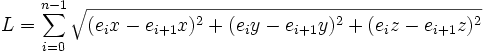$L = \sum_{i=0}^{n - 1}\sqrt{(e_ix-e_{i+1}x)^2 + (e_iy-e_{i+1}y)^2+(e_iz-e_{i+1}z)^2}$
Euclidean Length	Straight line distance between the endpoints of a trace	$D = \sqrt{(e_{1x}-e_{2x})^2 + (e_{1y}-e_{2y})^2+(e_{1z}-e_{2z})^2}$
Tortuousness	Also known as Fragmentation Smoothness or Contraction. Ratio of Path Length to Euclidean Distance ^[1]	$s= \frac{L}{D}$
Trace Density	The Average Spacing of Trace Bits	$\frac{L}{n}$
Volume	Volume is calculated by the local radius and path length	$V = \sum_{i=0}^{n - 1}\pi (r_i)^2*\sqrt{(e_ix-e_{i+1}x)^2 + (e_iy-e_{i+1}y)^2+(e_iz-e_{i+1}z)^2}$
Distance to parent	Separation of child traces to the parent	$D_p = \sqrt{(P_{1x}-C_{2x})^2 + (P_{1y}-C_{2y})^2+(P_{1z}-C_{2z})^2}$
Path to Root	Full path length to root	$\sum_{l=0}^{level}L_l$
	Merging Specific Features
Gap Size	Minimum distance between endpoints of two traces	$d= \sqrt{(x_1-x_2)^2+(y_1-y_2)^2+(z_1-z_2)^2}$
Angle	The angle created between two traces normalized as vectors	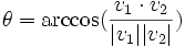$\theta = \arccos(\frac{v_1 \cdot v_2}{\|v_1\|\|v_2\|})$
Maximum Gap Distance	The maximum distance between endpoints that can be merged	$Δ$
Weights	The weights are used in the cost₁ algorithm	$α$ $β$
Cost₁	Weighted scalar evaluating the merge ^[2]	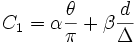$C_1=\alpha\frac{\theta}{\pi}+\beta\frac{d}{\Delta}$
Cost₂	Weighted scalar with Fragmentation Smoothness	$C_2=\theta[\frac{d}{\Delta}]s$
Curvature	The Hessian matrix for checking branching point existence and interpolating the path.	$\left[\begin{array}{ccc} f(x)_{xx}(X) + \frac{\alpha}{2}f_{yy}(X) + \frac{\alpha}{2}f_{zz}(X) & (1-\alpha)f_{xy}(X) & (1-\alpha)f_{xz}(X) \\ (1-\alpha)f_{xy}(X) & f_{yy}(X) + \frac{\alpha}{2}f(x)_{xx}(X) +\frac{\alpha}{2}f_{zz}(X) & (1-\alpha)f_{yz}(X) \\ (1-\alpha)f_{xz}(X) & (1-\alpha)f_{yz}(X) & f_{zz}(X) + \frac{\alpha}{2}f(x)_{xx}(X) +\frac{\alpha}{2}f_{yy}(X) \end{array} \right]$

Cell Features

Segments
- Total number of Traces in the Tree
Stems
- Number of Processes attached to Soma
Branch Pt
- How many branches in the cell
Leaf Nodes
- Total number of terminal tips
Leaf Level
- Number of compartments in the cells
Leaf Path Length
- Terminal path length
Total Euclidean Length
- Sum of all compartment euclidean lengths
Total Path Length
- Sum of all compartment path lengths
Average Segment path length
- Average path lengths of the compartments
Total Volume
- Sum of Volume of each compartment

We are currently working on integrating further with L-Measurefor a more detailed cell analysis.

Algorithms

Merge Small Gaps

Goal: Create longest continuous trace segments by merging close endpoints
Methods: Nearest neighbors  (Closest end points), 
Rejection based on conflicts and thresholds

Minimal distance between end points
- Angle between traces The angle is measured between the two traces by computing the norm of their vectors and the dot product.
  The equation is: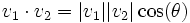 $v_1 \cdot v_2 = |v_1||v_2| \cos(\theta)$ which when solved for $θ$ is: $\theta = \arccos(\frac{v_1 \cdot v_2}{|v_1||v_2|})$
- Path length The path length is considered if the end points are not the best fit for the merge. For instance, a merging that would cause a sharp peak in the neurite. This is a more serious problem for large gaps (see below). To help alleviate this for small gaps, merge at the point where the direction changes sharply.
- Gap distance is too large The distance between the two points e_1, e_2 is computed to save computation. If the distance is longer than the excepted small gap distance, then the traces will not be considered for merging. A cost function adapted from "Automated Three-Dimensional Tracing of Neurons in Confocal and Brightfield Images" will take into account small gaps with two end points.
- Consider possibility of loops Though less probable in 3D, often there are 2D projections of 3D images resulting in loops being in the images. Loops in the branching structure can be avoided by checking the parents, Each of the trace Lines should have unique root nodes.
Another trace is a better fit (Cost Function)
- Smallest gap
- Better Angular alignment
"Bad merge"
- The merge causes corners
- Needs to be smoothed

Illustration of reconnecting fragmented structures using a cost algorithm on the critical points. The critical points 'a' and 'b' are merged because the cost C_(a,b) is less than the cost of merging other points. Point 'd' is rejected because its gap distance is beyond the threshold.^[2]

The Cost function we have implemented is modified from:
$C_1=\alpha\frac{\theta}{\pi}+\beta\frac{d}{\Delta}$
to include fragmentation smoothness. The original function had user selectable weights $α,β$ to scale the effects of the gap distance and angle of the merge. The Fragmentation smoothness is the ratio of the path distance to the end point displacement. If the merged traces start forming a "U" shape or a loop it would result in a higher cost. A second alteration is to multiply the factors so that the outliers are further differentiated from the more probable traces. The resulting formula:
$C_2=\theta[\frac{d}{\Delta}]s$
accounts for the three factors of angle, gap distance, and smoothness of the trace.

Interpolate Large Gaps

Goal: Connect Large gaps that step 1 cannot  simply connect by addition of a  single cell
Method: Larger gaps need new segments created, 
new Trace Bits must be added using manual tracing in the 3D cursor toolbox

Example showing how Merging and branching are interconnected. The Merging that creates sharp turns needs to be smoothed. The Traces need to create a new branch point and trace bits to interpolate the original path of the branch.

Branch Points

Goal: Detect and control Branching
Method: Detect most probable intercepts, 
Determination of main branch and child, 
Type of branch point

Distance maps
- Nearest neighbors (traces)
- Closest trace bits
Angle of intercept
Interpolation

Detect most probable intercepts: So far most of the methods I have evaluated or developed require information about the intensities in order to compute the most probable intercept. The reasoning behind this is the direction of the child branch does not give information about the intercept over long distances. In the short distance branching case, it is more acceptable to use the direction to figure out the interception point. The child branch would have to curve faster( over a shorter distance) if the direction of the branch was not in line with the main branch. In the case of a large gap between the main and child branch the child can curve slowly and still reach the main branch. This means that when there is a large gap there is more variation in the location of the intersection. So, to determine the proper intersection we can use the H(x) matrix listed in the features. I think when the gap is small( not sure what this is yet) we can just fill with a shortest distance line.

Soma Detection

Goal: Correspond processes with a soma
Method: Segmentation of original data, 
Localize the area to attach processes to soma, 
Correct direction of traces

Image intensity
Blob segmentation
Centroid
Distance map
Connectivity
- Connected components
- Localization of processes

Illustration of how the processes should be connected to a soma(shown in red).
The Dendrites are shown in blue, where the axon is shown in yellow.

Fragments

Goal: Removal of small traces that do not correspond to a process
Method: Small traces removed, 
Leftovers from splitting operators, 
Line fragments that cannot be merged

Lowest percentile of length
- Traces with no parents or children
- Type dependent

References

↑ Ascoli, Generation,Description and Storage of Dendritic Morphology Data
↑ ^2.0 ^2.1 Wenyun He, Automated Three-Dimensional Tracing of Neurons in Confocal and Brightfield Images

[Ascoli-0] Ascoli, Generation,Description and Storage of Dendritic Morphology Data

[Wenyun-1] 2.0 ^2.1 Wenyun He, Automated Three-Dimensional Tracing of Neurons in Confocal and Brightfield Images

[1]

[2]

Trace Editor/Features

Contents