SuperEllipseTrace3D
| Line 12: | Line 12: | ||
the medial axis of each vessel in the vasculature. Another key advantage when using the superellipsoid model is that its local nature allows us to adapt vessel intensity estimates across different regions of the vasculature. | the medial axis of each vessel in the vasculature. Another key advantage when using the superellipsoid model is that its local nature allows us to adapt vessel intensity estimates across different regions of the vasculature. | ||
| + | '''Vascular local shape modelling using superellipsoid ''' | ||
[[Image:se_model.png |thumb|800px|'''Figure1:''' Shows the boundary of a superellispoid while the shape parameter <math> \epsilon_{1} </math> is varied between 1.0 and 0.25 and <math> \epsilon_{2} </math> is set to 1.|center]] | [[Image:se_model.png |thumb|800px|'''Figure1:''' Shows the boundary of a superellispoid while the shape parameter <math> \epsilon_{1} </math> is varied between 1.0 and 0.25 and <math> \epsilon_{2} </math> is set to 1.|center]] | ||
| Line 19: | Line 20: | ||
in early computer vision literature [2]. Superellipsoids are expressed implicitly as: | in early computer vision literature [2]. Superellipsoids are expressed implicitly as: | ||
| + | [[Image:seWorldGeometry.png |thumb|400px|'''Figure2:''' |right]] | ||
<math> | <math> | ||
\left(\left|x\right|^{\frac{2}{\epsilon_{2}}}+\left|y\right|^{\frac{2}{\epsilon_{2}}}\right)^{\frac{\epsilon_{2}}{\epsilon_{1}}}+\left|z\right|^{\frac{2}{\epsilon_{1}}}=1, | \left(\left|x\right|^{\frac{2}{\epsilon_{2}}}+\left|y\right|^{\frac{2}{\epsilon_{2}}}\right)^{\frac{\epsilon_{2}}{\epsilon_{1}}}+\left|z\right|^{\frac{2}{\epsilon_{1}}}=1, | ||
| Line 27: | Line 29: | ||
the shape parameters, first note that with <math> \epsilon_{1}=\epsilon_{2}=1 </math> equation 1 is simply an ellipsoid. With <math>\epsilon_{1}\leq </math> and <math>\epsilon_{2}= 1</math> the superellipsoid becomes a cylindroid, i.e., the implicit surface bounds a convex region, where for constant <math>z</math>, the 2-D level curves are | the shape parameters, first note that with <math> \epsilon_{1}=\epsilon_{2}=1 </math> equation 1 is simply an ellipsoid. With <math>\epsilon_{1}\leq </math> and <math>\epsilon_{2}= 1</math> the superellipsoid becomes a cylindroid, i.e., the implicit surface bounds a convex region, where for constant <math>z</math>, the 2-D level curves are | ||
elliptical. Setting <math>\epsilon_{1},\epsilon_{2}</math> to other values produces a variety of shapes including cuboids and pinched cuboids [2]. Since the goal in this work is to find an approximation to an elliptical cylinder, we will restrict our focus to cylindroidal forms. This means that <math>\epsilon_{2}</math> in equation is set to unity. | elliptical. Setting <math>\epsilon_{1},\epsilon_{2}</math> to other values produces a variety of shapes including cuboids and pinched cuboids [2]. Since the goal in this work is to find an approximation to an elliptical cylinder, we will restrict our focus to cylindroidal forms. This means that <math>\epsilon_{2}</math> in equation is set to unity. | ||
| + | |||
Starting with a set of points in the set | Starting with a set of points in the set | ||
| Line 51: | Line 54: | ||
| − | ''' | + | '''Robust Vascular Intensity model''' |
| + | A class of robust estimators known as ''M-estimates'' can be defined as any solution <math>T_{n}</math> to: | ||
| + | <math> | ||
| + | \sum_{i = 1}^{n}\psi(x_{i};T_{n})=0. | ||
| + | </math> | ||
| + | |||
| + | |||
| + | The notation <math>T_{n}</math> refers to the dependency of the | ||
| + | estimate on a finite i.i.d. sample, <math>\{X_{1},X_{2},...,X_{n}\}</math>, | ||
| + | i.e., <math>T_{n}=T_{n}(X_{1},X_{2},...,X_{n})</math>. | ||
| + | |||
| + | When estimating the background, the main challenge is to deal with | ||
| + | the fact that the image data invariably contains vessel, | ||
| + | background clutter, and uncorrelated noise. Taken as a whole, the | ||
| + | resulting image data is a mixture of various components. Finding | ||
| + | the single component corresponding to the background region can be | ||
| + | difficult. | ||
| + | |||
| + | This is especially true since the actual background voxels may not | ||
| + | be a majority population in the mixture. This often happens when a | ||
| + | small vessel is adjacent to a very large one. Hence, the median | ||
| + | may no longer be a good choice. The real problem in this case is | ||
| + | that when estimating the background one must deal with | ||
| + | pseudo-outliers, i.e., data that appears as an outlier to | ||
| + | the current process but might be an inlier to another process. For | ||
| + | example an adjacent vessel appears as an outlier when estimating | ||
| + | the local background intensity. However, the data is actually an | ||
| + | inlier to the adjacent vessel. | ||
| + | |||
| + | To deal with these outliers, we propose the \textit{skipped | ||
| + | median} which simply restricts the support of the signum function, | ||
| + | thereby excluding very large residuals from the intensity | ||
| + | estimate. The corresponding <math>psi</math>-function is given by: | ||
| + | |||
| + | <math> | ||
| + | \psi_{med(s)}=\text{sgn}(r) \times | ||
| + | 1_{[-s,s]}(r)=\left\{\begin{array}{r}\text{sgn}(r),|r|\leq | ||
| + | s\\0,|r|>s\end{array}\right.. | ||
| + | </math> | ||
| + | |||
| + | |||
| + | ''' Generalized likelihood ratio test''' | ||
When estimating the superellipsoid model parameters we will assume | When estimating the superellipsoid model parameters we will assume | ||
that a vessel segment consists of two piece-wise constant regions | that a vessel segment consists of two piece-wise constant regions | ||
| Line 79: | Line 123: | ||
boundary using a gradient search. The following two subsections will detail each step. | boundary using a gradient search. The following two subsections will detail each step. | ||
| + | '''Traversing Vessels Using the | ||
| + | Superellipsoid ''' | ||
| + | |||
| + | [[Image:seTraversal.png |thumb|400px|'''Figure3: Illustrating vessel traversal. Figure shows a sequence of | ||
| + | superellipsoidal fits denoted <math>k</math>, <math>k+1</math>, and <math>k+2</math> superimposed | ||
| + | on a vessel. Note that the traversal is directed using the local | ||
| + | pose to determine the next step in the traversal.''' |left]] | ||
| − | |||
| − | |||
[[Image:SeTraceExample.png |thumb|1200px|'''Figure4:''' |center]] | [[Image:SeTraceExample.png |thumb|1200px|'''Figure4:''' |center]] | ||
Revision as of 15:49, 11 May 2009
This page presents automated methods for robust modeling and analysis of 3-D vascular images using a \textit{cylindroidal superellipsoid} to model localized segments of vasculature. The proposed vessel model has an explicit, low-order parameterization, allowing for joint estimation of boundary and centerline information, thereby approximating the medial axis of tubular structures. Further, this explicit parameterization provides a geometric framework for traversing vessels in a directed manner. Topological information like branch point location and connectivity can also be detected as a side effect. An M-estimators provide robust region-based statistics that are used to drive the superellipsoid toward a vessel boundary. The proposed methodology behaves quite well across scale-space, shows a high degree of insensitivity to adjacent structures and implicitly handles branching.
Contents |
Local vascular modelling using Superellipsoid
The superellipsoid provides the basis for a simple shape model that describes localized vessel segments. It has an explicit low-order parameterization relating directly to the local pose of a vessel segment. Using this geometric information, it is straightforward to traverse entire vascular networks.Also, since the superellipsoid model furnishes joint estimates of the boundary and centerpoint of a vessel, the resulting traversal approximates the medial axis of each vessel in the vasculature. Another key advantage when using the superellipsoid model is that its local nature allows us to adapt vessel intensity estimates across different regions of the vasculature.
Also, since the superellipsoid model furnishes joint estimates of the boundary and centerpoint of a vessel, the resulting traversal approximates the medial axis of each vessel in the vasculature. Another key advantage when using the superellipsoid model is that its local nature allows us to adapt vessel intensity estimates across different regions of the vasculature.
Vascular local shape modelling using superellipsoid

Superellipsoids are geometric modeling primitives first introduced
in early computer vision literature [2]. Superellipsoids are expressed implicitly as:

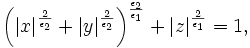
where the parameters  control the shape of the superellipsoid. To understand the role of
the shape parameters, first note that with ε1 = ε2 = 1 equation 1 is simply an ellipsoid. With
control the shape of the superellipsoid. To understand the role of
the shape parameters, first note that with ε1 = ε2 = 1 equation 1 is simply an ellipsoid. With  and ε2 = 1 the superellipsoid becomes a cylindroid, i.e., the implicit surface bounds a convex region, where for constant z, the 2-D level curves are
elliptical. Setting ε1,ε2 to other values produces a variety of shapes including cuboids and pinched cuboids [2]. Since the goal in this work is to find an approximation to an elliptical cylinder, we will restrict our focus to cylindroidal forms. This means that ε2 in equation is set to unity.
and ε2 = 1 the superellipsoid becomes a cylindroid, i.e., the implicit surface bounds a convex region, where for constant z, the 2-D level curves are
elliptical. Setting ε1,ε2 to other values produces a variety of shapes including cuboids and pinched cuboids [2]. Since the goal in this work is to find an approximation to an elliptical cylinder, we will restrict our focus to cylindroidal forms. This means that ε2 in equation is set to unity.
Starting with a set of points in the set
 (ε
is fixed), a transformation given by
(ε
is fixed), a transformation given by
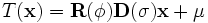 can be performed. This transformation preserves orthogonality of
the local coordinate frame while allowing for anisotropic scaling.
The action of
can be performed. This transformation preserves orthogonality of
the local coordinate frame while allowing for anisotropic scaling.
The action of  is to first scale
  by
by
 , which is a
  matrix with
scale parameters
matrix with
scale parameters
 on the
diagonal. Then, a rotation is performed via the matrix
on the
diagonal. Then, a rotation is performed via the matrix
 with three degrees of freedom that is
parameterized by φ. Finally, a shift via
with three degrees of freedom that is
parameterized by φ. Finally, a shift via
 is performed.
This transformation leads to a new superellipsoid defined by the
set having 10 degrees of freedom in 3D,
is performed.
This transformation leads to a new superellipsoid defined by the
set having 10 degrees of freedom in 3D,
 ,
where,
,
where,

Robust Vascular Intensity model
A class of robust estimators known as M-estimates can be defined as any solution Tn to:
The notation Tn refers to the dependency of the
estimate on a finite i.i.d. sample, {X1,X2,...,Xn},
i.e., Tn = Tn(X1,X2,...,Xn).
When estimating the background, the main challenge is to deal with the fact that the image data invariably contains vessel, background clutter, and uncorrelated noise. Taken as a whole, the resulting image data is a mixture of various components. Finding the single component corresponding to the background region can be difficult.
This is especially true since the actual background voxels may not be a majority population in the mixture. This often happens when a small vessel is adjacent to a very large one. Hence, the median may no longer be a good choice. The real problem in this case is that when estimating the background one must deal with pseudo-outliers, i.e., data that appears as an outlier to the current process but might be an inlier to another process. For example an adjacent vessel appears as an outlier when estimating the local background intensity. However, the data is actually an inlier to the adjacent vessel.
To deal with these outliers, we propose the \textit{skipped median} which simply restricts the support of the signum function, thereby excluding very large residuals from the intensity estimate. The corresponding psi-function is given by:
![\psi_{med(s)}=\text{sgn}(r) \times
1_{[-s,s]}(r)=\left\{\begin{array}{r}\text{sgn}(r),|r|\leq
s\\0,|r|>s\end{array}\right..](/mw/images/math/8/3/0/8308541e0e73f1216b90c2fd180e1adf.png)
Generalized likelihood ratio test
When estimating the superellipsoid model parameters we will assume
that a vessel segment consists of two piece-wise constant regions
with intensities denoted IF for foreground and IB for
background and that the vessel boundary separating these regions
is well-modeled by a superellipsoid. The local vessel intensities are modeled using a homogeneous
grayscale appearance model as
![V(\mathbf{x};{\theta})= I_{B}-(I_{B}-I_{F})\times
1_{\left[S(\mathbf{x},{\beta})<1\right]},](/mw/images/math/8/c/d/8cd0142b47915c3afacc0233da5ab6fb.png)
where  is the full parameter set of the superellipsoid vessel model. This
includes the intensity parameters
is the full parameter set of the superellipsoid vessel model. This
includes the intensity parameters  that
describe the foreground and background intensities respectively,
as well as the underlying parameters of the superellipsoid shape
model, i.e.,
that
describe the foreground and background intensities respectively,
as well as the underlying parameters of the superellipsoid shape
model, i.e.,  .
The notation
.
The notation ![1_{\left[\cdot\right]}](/mw/images/math/c/a/6/ca63e2b96befb2ce2cd7c85dfd2f4e93.png) denotes an indicator
function that evaluates to one on the set specified in the
subscript and is zero elsewhere.
denotes an indicator
function that evaluates to one on the set specified in the
subscript and is zero elsewhere.
The strategy for maximizing equation is to alternate between estimating the intensity parameters and then updating the
boundary using a gradient search. The following two subsections will detail each step.
Traversing Vessels Using the Superellipsoid

