SuperEllipseTrace3D
This page presents automated methods for robust modeling and analysis of 3-D vascular images using a cylindroidal superellipsoid to model localized segments of vasculature[1]. The proposed vessel model has an explicit, low-order parameterization, allowing for joint estimation of boundary and centerline information, thereby approximating the medial axis of tubular structures. Further, this explicit parameterization provides a geometric framework for traversing vessels in a directed manner. Topological information like branch point location and connectivity can also be detected as a side effect. An M-estimators provide robust region-based statistics that are used to drive the superellipsoid toward a vessel boundary. The proposed methodology behaves quite well across scale-space, shows a high degree of insensitivity to adjacent structures and implicitly handles branching.
Contents |
Local vascular modelling using Superellipsoid
The superellipsoid provides the basis for a simple shape model that describes localized vessel segments. It has an explicit low-order parameterization relating directly to the local pose of a vessel segment. Using this geometric information, it is straightforward to traverse entire vascular networks.Also, since the superellipsoid model furnishes joint estimates of the boundary and centerpoint of a vessel, the resulting traversal approximates the medial axis of each vessel in the vasculature. Another key advantage when using the superellipsoid model is that its local nature allows us to adapt vessel intensity estimates across different regions of the vasculature. Also, since the superellipsoid model furnishes joint estimates of the boundary and centerpoint of a vessel, the resulting traversal approximates the medial axis of each vessel in the vasculature.
Vascular local shape modelling using superellipsoid

Superellipsoids are geometric modeling primitives first introduced
in early computer vision literature [2]. Superellipsoids are expressed implicitly as:

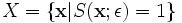
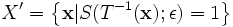
![\left[\mathbf{P}_{1},\mathbf{P}_{2},\mathbf{P}_{3}\right]](/mw/images/math/3/d/3/3d390fda91c51e931c61add349f094f7.png) . The dark ellipse oriented relative to the principal axes indicates the local vessel boundary and is labelled with the vessel cross-sectional scale values σ1 and σ2. The line labelled σ3 describes the approximate length over which the vessel segment is locally cylindriodal.
. The dark ellipse oriented relative to the principal axes indicates the local vessel boundary and is labelled with the vessel cross-sectional scale values σ1 and σ2. The line labelled σ3 describes the approximate length over which the vessel segment is locally cylindriodal.
where the parameters ε = (ε1,ε2) control the shape of the superellipsoid. To understand the role of the shape parameters, first note that with ε1 = ε2 = 1 equation of superellipsoid is simply an ellipsoid. With ε1 < = 1 and ε2 = 1 the superellipsoid becomes a cylindroid, i.e., the implicit surface bounds a convex region, where for constant z, the 2-D level curves are elliptical. Setting ε1,ε2 to other values produces a variety of shapes including cuboids and pinched cuboids [2]. Since the goal in this work is to find an approximation to an elliptical cylinder, we will restrict our focus to cylindroidal forms. This means that ε2 in equation is set to unity.
Starting with a set of points in the set
 (ε
is fixed), a transformation given by
(ε
is fixed), a transformation given by
 can be performed. This transformation preserves orthogonality of
the local coordinate frame while allowing for anisotropic scaling.
The action of
can be performed. This transformation preserves orthogonality of
the local coordinate frame while allowing for anisotropic scaling.
The action of  is to first scale
  by
by
 , which is a
  matrix with
scale parameters
matrix with
scale parameters
 on the
diagonal. Then, a rotation is performed via the matrix
on the
diagonal. Then, a rotation is performed via the matrix
 with three degrees of freedom that is
parameterized by φ. Finally, a shift via
with three degrees of freedom that is
parameterized by φ. Finally, a shift via
 is performed.
This transformation leads to a new superellipsoid defined by the
set having 10 degrees of freedom in 3D,
is performed.
This transformation leads to a new superellipsoid defined by the
set having 10 degrees of freedom in 3D,
 ,
where,
,
where,

Robust Vascular Intensity model
When estimating the background, the main challenge is to deal with the fact that the image data invariably contains vessel, background clutter, and uncorrelated noise. Taken as a whole, the resulting image data is a mixture of various components. Finding the single component corresponding to the background region can be difficult.
This is especially true since the actual background voxels may not be a majority population in the mixture. This often happens when a small vessel is adjacent to a very large one. Hence, the median may no longer be a good choice. The real problem in this case is that when estimating the background one must deal with pseudo-outliers, i.e., data that appears as an outlier to the current process but might be an inlier to another process. For example an adjacent vessel appears as an outlier when estimating the local background intensity. However, the data is actually an inlier to the adjacent vessel.
To deal with these outliers, we propose the skipped median which simply restricts the support of the signum function of the M-Estimator, thereby excluding very large residuals from the intensity estimate. The corresponding psi-function is given by:
![\psi_{med(s)}=\text{sgn}(r) \times
1_{[-s,s]}(r)=\left\{\begin{array}{r}\text{sgn}(r),|r|\leq
s\\0,|r|>s\end{array}\right..](/mw/images/math/8/3/0/8308541e0e73f1216b90c2fd180e1adf.png)
where the cutoff value is chosen as  .
.
When estimating the superellipsoid model parameters we will assume
that a vessel segment consists of two piece-wise constant regions
with intensities denoted IF for foreground and IB for
background and that the vessel boundary separating these regions
is well-modeled by a superellipsoid. The local vessel intensities are modeled using a homogeneous
grayscale appearance model as
![V(\mathbf{x};{\theta})= I_{B}-(I_{B}-I_{F})\times
1_{\left[S(\mathbf{x},{\beta})<1\right]},](/mw/images/math/8/c/d/8cd0142b47915c3afacc0233da5ab6fb.png)
where  is the full parameter set of the superellipsoid vessel model. This
includes the intensity parameters
is the full parameter set of the superellipsoid vessel model. This
includes the intensity parameters  that
describe the foreground and background intensities respectively,
as well as the underlying parameters of the superellipsoid shape
model, i.e.,
that
describe the foreground and background intensities respectively,
as well as the underlying parameters of the superellipsoid shape
model, i.e.,  .
The notation
.
The notation ![1_{\left[\cdot\right]}](/mw/images/math/c/a/6/ca63e2b96befb2ce2cd7c85dfd2f4e93.png) denotes an indicator
function that evaluates to one on the set specified in the
subscript and is zero elsewhere.
denotes an indicator
function that evaluates to one on the set specified in the
subscript and is zero elsewhere.
The strategy for maximizing equation is to alternate between estimating the intensity parameters and then updating the
boundary using a gradient search. The following two subsections will detail each step.
Generalized likelihood ratio test
Consider the image data
 with discrete domain
  and
the hypothesis pair:
and
the hypothesis pair:
![H_{0}:I(\mathbf{x})= I_{B}+N;
H_{1}:I(\mathbf{x})= I_{B}-(I_{B}-I_{F})\times
1_{\left[S(\mathbf{x},{\beta})<1\right]} + N.](/mw/images/math/5/0/d/50d7b76fed6595fdb7378366f3c2932d.png)
Here, H0 is the hypothesis that the image data is from the background process centered at IB and corrupted by independent identically distributed (i.i.d) noise denoted N with marginal distribution f. The alternative, H1, is the hypothesis that the image data contains a vessel that is well-modeled by the superellipsoid model given in equation.
Traversing Vessels Using Superellipsoid

The algorithm for traversing entire vascular networks using the local superellipsoid model is given as follows
- Extract a set of candidate seeds
- for each seed point
- Fit an initial superellipsoid
- Traverse the vessel in the forward direction by shifting the model center in the direction of the major axis;
- Refine the parameter estimates from the previous step;
- When the forward traversal terminates, restart the procedure in the reverse direction.
- select next seed point
Shown in Figure 4 is an example of the algorithm run on a sample dataset.
Software Usage
Use the trace 3D package from Farsight and type the following in command line
Trace3D.exe [ImageFileName] [Xml Parameter file]
where
- ImageFileName should the name of the file containing the 3D image (like tif, pic, lsm)
- XML parameter file is an XML file containing all the necessary Parameters and Data to run the software.
Input Parameter XML file
  <?xml version="1.0" ?>
  <SuperElliposoidTracing >
     <Parameter UseMultiscaleHessianFilter = "1" />
     <Parameter GridSpacing = "20" />
     <Parameter StepRatio = "0.5" />
     <Parameter MaxModelAspectRatio = "2.5" />
     <Parameter THRESHOLD = "0.3" />
     <Parameter XYSpacing = "0.7" />
     <Parameter ZSpacing = "1.0" />
     <Parameter minContrast = "3.0" />
     <Parameter StartTHRESH = "0.3" />
     <Parameter StartIterations = "100" />
     <Data InputFileName="C:\Data\myFirstImage.tiff" OutputFileName="C:\Results\myFirstImage.xml" />
     <Data InputFileName="C:\Data\mySecondImage.tiff" OutputFileName="C:\Results\mySecondImage.xml" />
     <Data InputFileName="C:\Data\myThirdImage.tiff" OutputFileName="C:\Results\myThirdImage.xml" />
  </SuperElliposoidTracing>
| Parameter Name | Description | Range(Default) |
|---|---|---|
| UseMultiscaleHessianFilter | This parameter when set to 1 performs a multi-scale Hessian filtering of the data prior to tracing. Multi-scale Hessian filtering enhances the tubular structures in the image selectively, and aids in their recovery from noisy images. However, this filter requires additional memory and is not recommended for very large size images. | 0 - no filtering, 1 - filtering |
| GridSpacing | Grid spacing indicates the spacing between seed points detected in step 1. For a dense network this parameter value should be between 10 and 20, for a sparse network this parameter value can be upto 50 or 70. | (15 to 70) default = 15 pixels |
| StepRatio | After each iteration, the Superellipsoid advances by an amount that is given by StepRatio x average scale of the vessel. | 0.1 to 1 (default = 0.5) |
| MaxModelAspectRatio | This the ratio of maximum allowable deformation between the largest cross section and the axial dimension of the superellipsoid. | 1.5 to 3 (default = 2) |
| THRESHOLD | This is the threshold of the Generalized likelihood test. | 0 to 1 (default = 0.5) |
| XYSpacing | This parameter specifies the resolution of the image in X and Y direction. The resolution is used in the computation of length of the vessels that is reported in the output statistics file. | |
| ZSpacing | This parameter specifies the resolution of the image in Z direction. The resolution is used in the computation of length of the vessels that is reported in the output statistics file. | |
| minContrast | The absolute difference between the foreground and background intensity estimate is denoted as contrast. This parameter provides a check that the foreground and background intensity estimates are at least separated by this value. | 1 to 255 (default = 3) |
| StartTHRESH | This is the threshold of the Generalized likelihood test for the seed detection step. In general this value is equal to THRESHOLD specified above. But in some noisy images, the user may like the tracing to start only from some high confidence seed points. In such a situation, StartTHRESH can be set to a value higher than THRESHOLD, and StartTHRESH would be used to start the tracing process and THRESHOLD would be used to terminate it. This provides a hysterisis effect canbe created between these two values. | 0 to 1 |
| StartIterations | Number of Iteration in the fitting process during seed detection. | default = 100 |
Each Data tag contains two parameters - Input Image file name and output XML file name. There can be many data tags in an input XML file, all of which is run sequentially with the settings specified by the parameter tag.
Output file format
The output of the program is an XML file that specifies all the parameters of the fitted sulerellipses. Shown below is a part of the example output format.There is a stand alone executable that allows a user to view, or Render Traces from an xml file without the rest of the farsight toolkit.
     <Superellipse ID="14833" TraceID="281" x="671.236607" y="258.665645" z="55.322431" a1="1.500000" a2="2.107491" a3="2.845113" q1="-0.682081" q2="0.200321" q3="0.694309" q4="0.112129" R11="0.010725" R12="0.125207" R13="0.992073" R21="0.431131" R22="0.894597" R23="-0.117565" R31="-0.902226" R32="0.428974" R33="-0.044386" Foregd="138.551697" Backgd="227.786545" Lhood="54.602578" MAD="25.525795">
          <Neighbor ID="14822" />
          <Neighbor ID="14834" />
     </Superellipse>
     <Superellipse ID="14821" TraceID="280" x="417.143258" y="435.645435" z="78.504042" a1="2.189383" a2="1.749069" a3="2.955666" q1="-0.617721" q2="0.242719" q3="0.727338" q4="0.174606" R11="-0.119016" R12="0.137361" R13="0.983345" R21="0.568793" R22="0.821201" R23="-0.045870" R31="-0.813824" R32="0.553860" R33="-0.175866" Foregd="17.251381" Backgd="231.372803" Lhood="16.683522" MAD="17.251381">
           <Neighbor ID="14820" />
     </Superellipse>
     <Superellipse ID="14820" TraceID="280" x="417.952850" y="435.050351" z="78.545288" a1="1.987939" a2="1.753001" a3="2.683718" q1="-0.608678" q2="0.271051" q3="0.725821" q4="0.170958" R11="-0.112085" R12="0.185352" R13="0.976259" R21="0.601585" R22="0.794610" R23="-0.081796" R31="-0.790906" R32="0.578135" R33="-0.200569" Foregd="32.018375" Backgd="230.739944" Lhood="18.919477" MAD="32.018375">
           <Neighbor ID="14819" />
           <Neighbor ID="14821" />
     </Superellipse>
     <Superellipse ID="14819" TraceID="280" x="418.700285" y="434.493639" z="78.595554" a1="1.850514" a2="1.848743" a3="2.498194" q1="-0.626554" q2="0.269445" q3="0.712833" q4="0.163395" R11="-0.069658" R12="0.179387" R13="0.981309" R21="0.588889" R22="0.801404" R23="-0.104697" R31="-0.805206" R32="0.570590" R33="-0.161463" Foregd="0.000000" Backgd="230.318024" Lhood="4.357347" MAD="7.383499">
           <Neighbor ID="14818" />
           <Neighbor ID="14820" />
     </Superellipse>
     <Superellipse ID="14818" TraceID="280" x="419.480872" y="433.934260" z="78.622114" a1="1.643896" a2="1.915647" a3="2.586124" q1="-0.665986" q2="0.233165" q3="0.690540" q4="0.158906" R11="-0.004193" R12="0.110362" R13="0.993883" R21="0.533678" R22="0.840766" R23="-0.091108" R31="-0.845678" R32="0.530031" R33="-0.062423" Foregd="0.000000" Backgd="229.685150" Lhood="48.524195" MAD="7.805420">
           <Neighbor ID="14817" />
           <Neighbor ID="14819" />
     </Superellipse>
     <Superellipse ID="14817" TraceID="280" x="420.319270" y="433.434016" z="78.606841" a1="1.504651" a2="1.951233" a3="2.634164" q1="-0.685737" q2="0.196658" q3="0.682080" q4="0.160804" R11="0.017818" R12="0.047734" R13="0.998701" R21="0.488812" R22="0.870935" R23="-0.050349" R31="-0.872207" R32="0.489074" R33="-0.007814" Foregd="0.000000" Backgd="229.474197" Lhood="47.535577" MAD="7.805405">
           <Neighbor ID="14816" />
           <Neighbor ID="14818" />
     </Superellipse>
     <Superellipse ID="14816" TraceID="280" x="421.179063" y="432.956243" z="78.617224" a1="1.500000" a2="1.967357" a3="2.655932" q1="-0.680289" q2="0.187983" q3="0.687879" q4="0.169386" R11="-0.003739" R12="0.028157" R13="0.999597" R21="0.489081" R22="0.871942" R23="-0.022732" R31="-0.872230" R32="0.488799" R33="-0.017031" Foregd="0.000000" Backgd="228.841324" Lhood="72.747855" MAD="8.227325">
           <Neighbor ID="14813" />
           <Neighbor ID="14817" />
     </Superellipse>
     <Superellipse ID="14812" TraceID="279" x="432.547160" y="1.497019" z="74.751805" a1="1.550276" a2="4.139033" a3="5.443840" q1="-0.570902" q2="-0.553356" q3="0.461459" q4="0.393604" R11="0.264262" R12="-0.960121" R13="0.091289" R21="-0.061284" R22="0.077746" R23="0.995088" R31="-0.962502" R32="-0.268559" R33="-0.038294" Foregd="159.858368" Backgd="235.802917" Lhood="27.702167" MAD="24.892929">
           <Neighbor ID="14811" />
     </Superellipse>
In the above description, "ID" refers to a specific fitted superellipse, "TraceID" refers to a traced segment, (x, y, z) refer to the center of the fitted superellipse, (a1, a2, a3) refer to the scale parameters of the superellipse along the 3 local coordinate axes. Specifically, a1 and a2 specify the elliptical cross-section, and a3 specifies the length of the superellipse. The parameters e1 and e2 specify the shape of the superellipse. The numbers (q1, q2, q3, q4) are the quaternion parameters. The 6 numbers (R11, R12,...R33) specify the rotation matrix. The foreground and background intensity estimates are specified by "foregd" and "Backgd" respectively. These are automatically inverted when necessary. Lhood refers to the likelihood ratio, and "MAD" refers to the median of absolute deviations as estimated by the model.
Graph to Tree conversion
Using the ConvertToSWC.exe, the XML graph structure can be converted in to a tree-structure (assuming the roots are known). We use SWC file convention to output the tree. An example of SWC file format is shown below.
     # File generated by Superellipse to SWC converter
     1 10 585.426 269.557 32.093 4.9308  -1
     2 10 587.979 269.277 32.8993 4.77079  1
     3 10 590.516 268.991 33.6324 4.66546  2
     4 10 593.03 268.721 34.334 4.64644  3
     5 10 595.484 268.467 35.0942 4.59934  4
     6 10 598.004 268.399 35.7682 4.66422  5
     7 10 600.506 268.38 36.4113 4.65517  6
     8 10 602.984 268.313 37.0774 4.65367  7
     9 10 605.467 268.125 37.7475 4.70399  8
References
[1] James Alexander Tyrrell, Emmanuelle di Tomaso, Danel Fuja, Ricky Tong, Kevin Kozak, Edward B. Brown, Rakesh Jain, Badrinath Roysam, “Robust 3-D Modeling of Vasculature Imagery Using Superellipsoids,” vol. 26, no. 2, pp. 223-237, IEEE Transactions on Medical Imaging, Feb 2007.
[2] Barr, A.H., "Superquadrics and Angle-Preserving Transformations," IEEE Computer Graphics and Applications, 1(1), pp. 11-23, 1981.
[3] K. Al-Kofahi, S. Lasek, D. Szarowski, C. Pace, G. Nagy, J. N.Turner, and B. Roysam, "Rapid automated three-dimensional tracing of neurons from confocal image stacks," IEEE Transactions on Information and Technology in Biomedicine, 6(2), pp. 171-187, 2002.
