Vessel Laminae Segmentation
This page describes the vessel surface segmentation algorithm. We provide the background, a brief description of the algorithm and show some sample results. Finally we provide instructions on how to run the program. As a note, this page describes only the key features of the algorithm. For a rigorous mathematical explanation the readers are encouraged to read the paper cited at the end.
Contents |
Background and motivation

Accurate and rapid segmentation of microvasculature from three-dimensional (3-D) images is important for diverse studies in neuroscience, tumor biology, stem-cell niches, cancer stem cell niches, and other areas. It is needed for measuring vascular features such as surface areas, diameters and tortuosities of vessel segments, branching patterns of the vascular tree, and distributions and orientations of cells relative to the vasculature. When time-lapse imaging of living vasculature is performed, segmentation results can be used for analyzing angiogenesis. Finally, quantifying the impact of pharmacological interventions requires vessel segmentation for change analysis.
Vessel segmentation algorithm presents a robust 3-D algorithm to segment vasculature that is image by labeling laminae, rather than lumenal volume. The signal is weak, sparse, noisy, non-uniform, low-contrast, and exhibits gaps and spectral artifacts, so adaptive thresholding & Hessian filtering based methods are not effective.
The Algorithm
The algorithm has four steps
- Basic surface extraction:
- Adaptive region growth:
- 3-D visualization and feature computation:
- Centerline extraction:
Basic surface extraction
The first step of our algorithm identifies high-confidence foreground voxels using a robust voxel-based generalized hypothesis test. Our test consists of two hypotheses. The hypothesis test is performed in a neighborhood Γ consisting of 7x7x7 voxels typically. A null hypothesis consists of voxels of uniform intensity λb. The alternate hypothesis consists of a cube of voxels of background intensity λ0 with a thick planar foreground region of intensity λ1 passing through the center voxel. We perform such a generalized likelihood ratio test on each voxel independently.
Adaptive region growth
The second step performs an adaptive region growing algorithm to identify additional foreground voxels while rejecting noise. The region growing criteria is based on the difference in background and foreground intensities identified in the first step. Starting at the high confidence voxels, we grow the voxels iteratively to neighboring regions with similar confidence. Iteration stops when no more voxels are left to be added. This step also yields relative estimates of detection confidence at each voxel.
3-D visualization and feature computation
The third step uses the marching tetrahedra algorithm to link the detected foreground voxels to produce a triangulated 3-D mesh with watertight isosurfaces. The mesh is smoothed using a volume-preserving algorithm to eliminate jagged facets, and adaptively decimated using an edge-collapsing and volume-preserving algorithm to produce the final mesh. Once this is complete, we estimate the local surface curvature at each triangle.

Segmented image
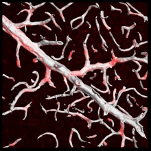
Segmentation overlaid on the raw image
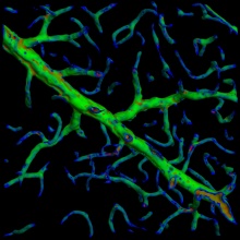
Confidence map over the segmentation
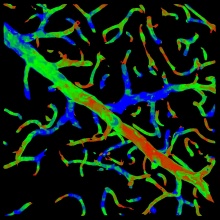
Curvatuve map over the segmentation


Centerline extraction

In this step, we compute a 'voted' image by casting rays uniformly from each point in the volume onto the 3-D mesh generated. The sum of all projections of the rays on the surface amounts to the vote at each point. The voting is performed on a subsampled image for efficiency and rays are limited in length. If no surface is found within the distance threshold, the ray's contribution to the vote is taken as zero. We run a conventional tube tracing algorithm on this output to generate a centerline image.
Validation
We employed an edit based validation technique. Validating a surface segmentation can be daunting task since mesh editing is a cumbersome one. We thus validated the effectiveness of our technique by using the extracted centerlines. Note that the errors due to tube tracing could add to the errors in the surface segmentation itself and we thus obtain only the cascaded error rate. A domain expert was provided with a editing tool capable of showing the raw data and the extracted centerlines simultaneously. The user could add or delete even parts of automatically computed segments. From these annotations, the average recall and precision were found to be 94.66% and 94.84%, respectively
Though limited in its effectiveness, we tried our algorithm on a phantom image data by adding Gaussian and Poisson noise to it. We found that our technique was quite robust and effective in such cases. For a more elaborate explanation of our findings, the reader is urged to refer to the original journal paper cited at the bottom of this page.
Parameters
For the real data sets used in our experiments, typical values are represented below along with some guidance on how to choose the parameters for a different application.
 : typical values: 8-12
Set this value high enough such that the segmentation detects at least some points in each vessel segment. One way to choose this is to set this equal to  and look at the points detected by the segmentation program. These are the initial points you expect to get detected. Choose this parameter before the lower threshold.
: typical values: 3-6
Set this value to a low enough value such that maximum vessel foreground points are detected.
ω : typical values: 1.5
This value is half the thickness of the vessels seen in the images(in voxels). Choose this based on the resolution of the imaging involved.
Γ size : typical values: 7x7x5
The neighborhood size used for doing hypothesis testing. Higher the neighborhood used, the more robust the test is and the less sensitive it is. Choosing higher neighborhood size also increases the computational time significantly.
Programs
C++ Code
The source code is available in the FARSIGHT svn repository under trunk/Vessel. Use CMake to configure and compile this code in any platform. Additional dependencies for this module apart from basic ones like ITK/VTK include OpenGL (v1.2+) and GLUT libraries. It is organized into four folders:
- Centerline - This folder contains source code for producing the 'filled' image used for generating the centerlines. This image is traced by common vessel tracing algorithms available in FARSIGHT.
- Common - This folder contains a common set of source codes for both visualizing and generating 'filled' vessel images.
- Segmentation - This folder contains source code for binarizing the raw vessel laminae image. It creates three kinds of files. (1) .npts files contains X,Y,Z locations of the binarized points along with L1,L2. L1 is the estimated difference in foreground and background intensity at that point and L2 is the computed likelihood ratio.
- Visualization - This folder contains source code (uses OpenGL libraries) to visualize the segmented vessels in 3D. The key bindings are as follows
- W - enables/disables wireframe mode
- V - enables/disables solid surfaces with lighting
- Left mouse button - enables 3-D rotation
- Right mouse button - enables zooming in and out of the 3-D vessel
Python Script
The segmentation code is also wrapped in python in FARSIGHT. For example, one can segment the image named 'NM_crop1_EBA.pic' and produce an output binary image 'NM_crop1_EBA_surface.pic' using the following command.
subprocess.call(['vessel_segmentation.exe', 'NM_crop1_EBA.pic', 'NM_crop1_EBA_surface.pic'])
For more details on how to run a demo file, see this excellent step-by-step tutorial - FARSIGHT Tutorials/5-Label
References
Arunachalam Narayanaswamy, Saritha Dwarakapuram, Christopher S. Bjornsson, Barbara M. Cutler, William Shain, Badrinath Roysam, Robust Adaptive 3-D Segmentation of Vessel Laminae from Fluorescence Confocal Microscope Images & Parallel GPU Implementation, (accepted, in press), IEEE Transactions on Medical Imaging, March 2009.