Trace Editor/Features
Contents |
Features and algorithms for Trace Editor
The Trace Editor uses several intrinsic and computed features in both manual and automated processes. Most features used for editing operate on the trace lines or the gap.
Feature List
| Feature | Description | Equation or Variable |
|---|---|---|
| Gap Size | Minimum distance between endpoints of two traces | 
|
| Angle | The angle created between two traces normalized as vectors | 
|
| Path Length | Total length along a trace, indicated by the size of the trace | 
|
| Euclidean Distance | Straight line distance between the endpoints of a trace | 
|
| Fragmentation Smoothness | Ratio of Path Length to Euclidean Distance [1] | 
|
| Maximum Gap Distance | The maximum distance between endpoints that can be merged | Δ |
| Weights | The weights are used in the cost algorithm | α β |
| Cost1 | Weighted scalar evaluating the merge | 
|
| Cost2 | Weighted scalar with Fragmentation Smoothness | ![C_2=\theta[\frac{d}{\Delta}]s](/mw/images/math/8/3/8/838dc6bcf55d56903864da4855c33cca.png)
|
| Curvature | The Hessian matrix for checking branching point existence and interpolating the path. (Still under consideration) | ![\left[\begin{array}{ccc}
f(x)_{xx}(X) + \frac{\alpha}{2}f_{yy}(X) + \frac{\alpha}{2}f_{zz}(X) & (1-\alpha)f_{xy}(X) & (1-\alpha)f_{xz}(X) \\
(1-\alpha)f_{xy}(X) & f_{yy}(X) + \frac{\alpha}{2}f(x)_{xx}(X) +\frac{\alpha}{2}f_{zz}(X) & (1-\alpha)f_{yz}(X) \\
(1-\alpha)f_{xz}(X) & (1-\alpha)f_{yz}(X) & f_{zz}(X) + \frac{\alpha}{2}f(x)_{xx}(X) +\frac{\alpha}{2}f_{yy}(X)
\end{array} \right]](/mw/images/math/8/6/2/86265c277f698370dbb9b8bbf95c9619.png)
|
| Parent | Considering nerves branching from the soma are a tree like structure, a parent point can be used to find a cycle. |
Algorithms
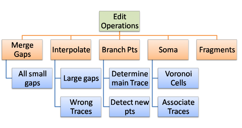
The algorithms suggested are used to control the editing process allowing for rule based cluster editing. The Goal is to complete group editing in five steps.
Merge Small Gaps
Goal: Create longest continuous trace segments by merging close endpoints
Methods: Nearest neighbors  (Closest end points),
Rejection based on conflicts and thresholds
- Minimal distance between end points
- Angle between traces- The angle is measured between the two traces by computing the norm of their vectors and the dot product.
The equation is: which when solved for θ is:
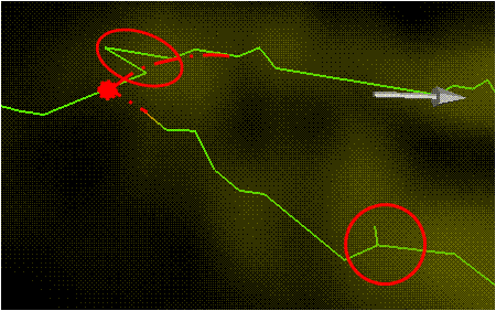
- Path length- The path length is considered if the end points are not the best fit for the merge. For instance, a merging that would cause a sharp peak in the neurite. This is a more serious problem for large gaps (see below). To help alleviate this for small gaps, merge at the point where the direction changes sharply.
- Gap distance is too large- The distance between the two points e_1, e_2 is computed to save computation. If the distance is longer than the excepted small gap distance, then the traces will not be considered for merging. A cost function adapted from "Automated Three-Dimensional Tracing of Neurons in Confocal and Brightfield Images" will take into account small gaps with two end points.
- Consider possibility of loops Though less probable in 3D, often there are 2D projections of 3D images resulting in loops being in the images. Loops in the branching structure can be avoided by checking the parents, as a trace cannot have two parents, but there can be two children.
- Angle between traces- The angle is measured between the two traces by computing the norm of their vectors and the dot product.
- Another trace is a better fit (Cost Function)
- Smallest gap
- Better Angular alignment
- "Bad merge"
- The merge causes corners
- Needs to be smoothed
The Cost function we have implemented is modified from: 
to include fragmentation smoothness. The Fragmentation smoothness is the ratio of the path distance to the end point displacement. If the merged traces start forming a "U" shape or a loop it would result in a higher cost. A second alteration is to multiply the factors so that the outliers are further differentiated from the more probable traces. The resulting formula:
![C_2=\theta[\frac{d}{\Delta}]s](/mw/images/math/8/3/8/838dc6bcf55d56903864da4855c33cca.png)
accounts for the three factors of angle, gap distance, and smoothness of the trace.
Interpolate Large Gaps
Goal: Connect Large gaps that step 1 cannot  simply connect by addition of a  single cell
Method: Larger gaps need new segments created,
new Trace Bits must be added,
smoothing operator.
- Curve fitting to find trend of:
- Direction
- Curvature
- Interpolation
- Extend the line
- Most probable vector
- Avoid creating edges
Branch Points
Goal: Detect and control Branching
Method: Detect most probable intercepts,
Determination of main branch and child,
Type of branch point
- Distance maps
- Nearest neighbors (traces)
- Closest trace bits
- Angle of intercept
- Interpolation
Detect most probable intercepts: So far most of the methods I have evaluated or developed require information about the intensities in order to compute the most probable intercept. The reasoning behind this is the direction of the child branch does not give information about the intercept over long distances. In the short distance branching case, it is more acceptable to use the direction to figure out the interception point. The child branch would have to curve faster( over a shorter distance) if the direction of the branch was not in line with the main branch. In the case of a large gap between the main and child branch the child can curve slowly and still reach the main branch. This means that when there is a large gap there is more variation in the location of the intersection. So, to determine the proper intersection we can use the H(x) matrix listed in the features. I think when the gap is small( not sure what this is yet) we can just fill with a shortest distance line.
Soma Detection
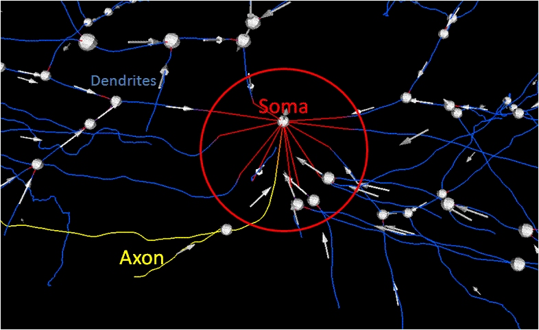
Goal: Correspond processes with a soma
Method: Segmentation of original data,
Localize the area to attach processes to soma,
Correct direction of traces
- Image intensity
- Blob segmentation
- Centroid
- Distance map
- Connectivity
- Connected components
- Localization of processes
Fragments
Goal: Removal of small traces that do not correspond to a process
Method: Small traces removed,
Leftovers from splitting operators,
Line fragments that cannot be merged
- Lowest percentile of length
- Traces with no parents or children
- Type dependent
References
- ↑ Ascoli, Generation,Description and Storage of Dendritic Morphology Data


