MDL Neuron Modeling

From FarsightWiki

The Minimum Description Length (MDL) principle was developed by Rissanen in 1978 and it has its root in information theory [1]. It was generated from Shannon’s classic statistical communication theory [2] and Solomonoff’s inductive inference theory [3]. The original idea is to minimize the codes in terms of binary digits (bits) of a signal to be sent over a communication channel and be decoded on the other side of the channel.

The MDL principle can provide a complete estimation of the parameter model, including not only the number of its components and the parameters themselves. With the MDL model of backbones at its optimal value, the whole dendritic model can be accomplished by comprising the spine model based on the MDL pinciple. The spine models are secondary structure of the whole dendritic model since they are attached to the backbones. Therefore, a minimum description tree (MDT) will be created.

If combining the cost function of two description length together, the description length of the minimum description tree includes the two parts: backbone model description and spine model description, which constitute the two levels of dendrite model.

1 Image Preprocessing Methods
- 1.1 Image Preprocessing
- 1.2 Anisotropic Diffusion
2 Grayscale Skeletonization of Dendrites and Spines
- 2.1 Gradient Vector Field and Critical Points
- 2.2 Creation of Skeletons
3 Graph Structure and Morphology
- 3.1 Minimum Spanning Tree with Intensity Weighted Edges
- 3.2 Graph Morphology Methods
4 MDL Method on Dendrites Structures
- 4.1 MDL on B-spline backbone models
5 MDL Method on Spines Structures
- 5.1 MDL on Dendritic Spine Structure
- 5.2 Spine Models with Prior Knowledge
6 Algorithm Parameters
7 Program Instruction
8 References

Image Preprocessing Methods

Upon the acquisition of deconvoloved confocal microscopy 3D images, the basic 3D image preprocessing methods, such as thresholding, morphological image processing, connected component removal and flood filling [4], are used for noise reduction, image enhancement and regions of interest (ROI) selection. Since the skeletonization method is based on 3D intensity images and corresponding gradient vector field, it is necessary to derive smooth vector field without the affection of noise, while still keeping the original intensity ridges.

Image Preprocessing

Thresholding
Morphological image processing
Connected component removal
Flood filling
Anisotropic diffusion

Anisotropic Diffusion

The algorithm used to extract the skeletons of the tubular objects is based on a computed gradient vector field with certain kernel. The original 3D intensity map contains noise corrupted part and it introduces irregular components to the gradient vector field. Therefore, it is necessary to smooth the 3D intensity map before deriving the vector field while it must preserve the ridges of neuronal structure at the same time.

Anisotropic diffusion can smooth out some unwanted small objects attached to the main part of the tubular objects, while it can overcome the edge shifting problem in isotropic linear diffusion. It is an iterative method that can produce smooth results while keeping useful edge structures [5].

Grayscale Skeletonization of Dendrites and Spines

Illustrating the graph generation procedure.

The gradient vector field is computed from the smoothed and regularized 3D images after the anisotropic diffusion. The skeletonization method is derived from the vector field where critical points and high curvature points are located as seed points. The central lines of neurons and spines are extracted by path-line formation along intensity ridges with all the necessary seed points.

Gradient Vector Field and Critical Points

Sobel kernel to compute vector field
Jacobian matrix of the vectors
Eigenvalues of Jacobian
Critical points
- Attracting points
- Repelling points
- Saddle points
High curvature points
- Here,the conception of curvature is iso-surface curface curvature for 3D image. For an image $u (x, y, z)$ , considering an iso-surface denote by $\sum$ ,let $\textbf{t}$ be any unit vector in the tangent plane $T p$ at a point $\textbf{p}$ and $\textbf{g}$ the normal to the surface at $\textbf{p}$ . Then the curvature at a point $\textbf{p}$ in the any unit vector $\textbf{t}$ can be defined by : 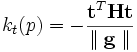$k_t(p) = - \frac{\textbf{t}^T \textbf{Ht}}{\parallel \textbf{g} \parallel}$ ,here $\textbf{H}$ is the Hessian Matrix of a 3D image function, $\textbf{g}$ is the gradient vector.Let $\textbf{t1}$ and $\textbf{t2}$ denote the two mutual orthogonal tangent directions whose curvatures are maximum and minimum, then the associated curvatures $k 1$ and $k 2$ are called principle curvature. Strictly speaking, to compute the principle curvature, we must first compute the principle direction. However, it can be proven that the principle curvature can be computed by the eigen-value of matrix $\textbf{He}$ , and $\textbf{He}$ is the sub-matrix (2x2)of the rotation Hessian matrix $\textbf{P}^T\textbf{HP}$ ,here $\textbf{P}$ is the rotation matrix to rotate the Hessian $\textbf{H}$ perpendicular to $\textbf{g}$ in the tangent plane.

Creation of Skeletons

The two kinds of seed points, saddles and high curvature points, constitute the starting points of flow integration. The iterative algorithm of path-line formation in vector fields move a step forward in the direction of the vector at each current position until the step size falls below a predetermined threshold. One can use a standard flow integration method to follow the path-lines [6]. Common integration schemes use either Euler schemes, Runge-Kutta second order (RK-2), or Runge-Kutta fourth order(RK-4).

Graph Structure and Morphology

In order to create connection relationships of skeleton points and make the dendrite and spine analyses easy to accomplish, a graph structure of the skeleton points needs to be constructed. The later MDL approaches are based on this graph model. Directly, the graph structure of dendritic backbones is obtained with a graph morphology method.

Minimum Spanning Tree with Intensity Weighted Edges

The skeleton points of dendrites and spines can be transformed into a graph structure that provides an easy way to manage the tree structure of neuron and it is straightforward to traverse the whole dendritic tree and measure the necessary data about it [7]. For instance, the graph can retrieve all the branch points immediately.

The vertices of graph are the whole 3D points of skeletons from streamline generation. Within curtain range of each point, graph edges are created and edge weights are computed based on point Euclidean distance and 3D image intensities.

Graph Morphology Methods

Dendrite tree model based on Graph
- The skeleton set produced by core-skeleton algorithm is just a initial skeleton,and it lacks an organization structure of component-wise differentiation. To distinguish skeletons that belong to backbone and those belong to spines, we first need to construct a weighted dendrite tree structure G=(V,E,W) to model the skeleton points,here V is the vertice set,E is the edge set and W is the weight map.For the skeletons on G, we will use Kruskal's Minimum Spanning Tree algorithm (KMST)to establish the effective connections among all the pairs of vertices. After KMST, a new Graph named G-MST can be constructed. And for the nodes on this graph, there are four types of vertices:isolated nodes with 0 degree,end nodes with 1 degree,curve nodes with 2 degree and branch nodes with more than 3 degree. Of our interest, we can extract two types of chains of edges based on the above knowledge:(1) Backbone chain, a chain that run between two branch nodes;(2) Branch chain, a chain that start at end node and end at a branch node.
MDL-based Estimation of Dendritic Backbone
- In order to extract backbone,Graph erosion operation will be used to remove unwanted trivial leaves of the tree and keep the major tree structure. After a sequence of erosion operations on the tree, original backbone structure will show up. However it is a little shorter than the true value, a dilation operation will bring it back to its original length.

MDL Method on Dendrites Structures

Four examples illustrating the qualitative improvement from using the MDL approach over a conventional skeletonization approach.

The structures of dendritic backbones can be approximately and concisely fitted by polynomial splines prior to any surface reconstruction if necessary. Currently, there are two commonly used ways, the piecewise polynomial form and B-spline form. With MDL principle, the best fitted B-spline functions can be achieved to be optimized backbone model. The MDL method can automatically and inherently prevent from overfitting and it can overcome the difficulty in estimation of both the parameters and the structure of a model that includes the number of parameters [8].

MDL on B-spline backbone models

The spline fitting was applied to real datasets. The original extracted dendritic backbone is not smooth at some places. They can be represented with piecewise B-Spline functions well. The order and complication of the B-spline model that is optimal can be determined by the MDL principle. On the one hand, simple spline functions don't fit the data well; on the other hand, high order spline functions are too complicated and have some unnecessary ripples.

MDL Method on Spines Structures

The data are described in terms of extracted features from the fluorescence Images. The features are assumed to be best representation of spines from both geometry and intensity properties of spines. The features under consideration are mean intensity of the branch, length of the branch, and mean vesselness of the branch, etc. The features are components of multi-dimensional vector space.

MDL on Dendritic Spine Structure

The descriptive language is based on feature descriptions and model description [9]. When the features are determined for each spine, the spine can be established. Assume the observed spine features are the sum of certain feature values and noise with some variances. These two components add up to the given feature observations exactly.

Spine Models with Prior Knowledge

Consider two factors in the prior distribution of spine models:

The relationship of neighborhood of spines on a dendrite;
The relationship of a spine with its dendritic backbone.

When prior knowledge comes into the model, more bits will be needed to describe additional information of the spines. Among other prior knowledge of dendritic structure, the first one is the spine local restriction. Assuming the neighboring two spines are not intending to be too close to each other; otherwise it can be a false detection. Under the other prior knowledge of spine positions on dendrites, the spines are protruding from backbones only and the protruding positions are not far from the backbone. Otherwise, it is not likely to be a spine. it can be called offbranch problem to restrict the spines not to be far away from the backbone lines.

Illustrating the improved spine detection after backbone smoothing on the images in the previous figure.

Algorithm Parameters

According to the discussion of the algorithm above, the main parameters of the algorithm are summarized in the following table. There are some variances among all the datasets, but within the same source of datasets, the selection of parameters has small ranges.

Parameter	Description	Typical range of values
Intensity threshold	Threshold value to identify pixels that are definitely part of the background that can be ignored for processing (use higher values for images with higher background intensities).	2 – 7 (based on background range)
Connected components size	Used to remove objects that are too small to be spines (use higher value to eliminate larger false objects due to imaging noise).	10 – 100
Anisotropic Diffusion conduction parameter k	Anisotropic diffusion conduction coefficient. (use higher value of this parameter to increase the amount of image smoothing).	10 – 800
Anisotropic Diffusion smoothing iterations t	Number of iterations of anisotropic diffusion smoothing (use larger number to guarantee convergence if necessary).	2 – 10
Gradient vector magnitude threshold for detecting critical	This is a threshold value used to choose critical points. When the image intensity gradient magnitude is lower than this threshold, a critical point is detected (use higher value to detect more critical points, i.e., increase sensitivity of critical point detection).	0.04 – 0.15
Threshold for detecting high curvature seed points	If the curvature at a point has a value above this threshold parameter, and it is also a local maximum of curvature values, we treat it as a high curvature seed point (use higher values to pick up fewer seed points)	0 – 10
IW-MST edge range threshold	If the distance between 2 vertices on the initial graph exceeds this threshold, we assume there is no edge between them in the graph structure before generating the IW-MST (use higher value to obtain a more connected graph).	5 – 15
Graph prune size	Threshold size used to prune the minimal spanning tree structure and eliminate trivial branches are shorter than this length (use a higher value for pruning longer branches).	2 – 10
Number of iterations for the graph morphology	The number of iterations of graph theoretic erosion and dilatation steps to clean up the IW-MST to estimate the neurite backbones. (use a higher value for eliminating longer small branches).	30 – 70
MDL weight factor α	Optional parameter to adjust the tradeoff between coverage and conciseness in the MDL estimation for spines only. (use a higher value for more complex models).	0.5 – 0.95
Extra spine detection offset	If the distance between the initially detected backbone (blue line) and the fitted spline (red line) exceeds this threshold, then we detect this missing spine (use a lower value for detecting more extra spines).	1.5

Program Instruction

Input file formats:

Raw images
Tiff images
LSM images (convert to raw images)

Output file formats:

SWC files
VTK files

For more details on how to run the code for this module, please visit the Program Instruction page

References

[1] J. Rissanen, Modeling by shortest data description, Automatica, vol. 14, no. 5, pp. 465-471, 1978.
[2] C.E., Shannon, W. Weaver, The Mathematical Theory of Communication, The University of Illinois Press, 1949.
[3] R.J. Solomonoff, A Formal Theory of Inductive Inference: Part I and II, Information and Control, 7, 1964, Part I: pp. 1-22, Part II: pp. 224-254.
[4] D.F. Rogers, Procedural Elements for Computer Graphics, McGraw-Hill, Boston, MA, 1998.
[5] P. Perona and J. Malik, “Scale-space and edge detection using anisotropic diffusion,” IEEE Trans. Pattern Anal. Machine Intell., vol. 12, no. 7 pp. 629–639, July 1990.
[6] W. Schroeder, K. Martin and B. Lorensen, The Visualization Toolkit an Object Oriented Approach to 3D Graphics, Printice-Hall, Inc., 1998.
[7] Cohen, A. R., Roysam, B., and Turner, J. N., Automated Tracing and Volume Measurements of Neurons from 3-D Confocal Fluorescence Microscopy Data, Journal of Microscopy, Vol. 173, Pt. 2, February 1994.
[8] P. Grunwald, J. Myung, and M. Pitt, Advances in Minimum Description Length: Theory and Applications, MIT Press, 2004.
[9] Y. G. Leclerc, Constructing simple stable descriptions for image partitioning, Int. J. Comput. Vision, vol. 3, no. 1, pp. 73-102, 1989.