User:Gilbes
Tensor Voting Framework:
Tensor Voting and Application
Sam Gilbert
Rensselaer Polytechnic Institute Masters of Engineering
Abstract:
The human vision system has an amazing ability to distinguish between background and foreground, signal from noise, and motion between frames, but replicating such distinctions in computer vision has proved to be quite difficult. One such replication method is Tensor voting (TV), which is adapted from Gestalt principles that outline how the human mind groups what it perceives to be similar objects by such things as shape, color, orientation, velocity, etc. In this paper I will address the original method developed in the early 1990’s, its key shortcomings in curvature segmentation, some of the recent adaptations developed to address these shortcomings, like iterative scaling, and the shortcomings of these adaptations, like the exponential increases in computation time.
1. Introduction of the Original Method of Tensor Voting and Its Drawbacks:
The process of creating a TV framework creates a matrix that is comprised of the orientation of the tangential at a pixel, the possibility that it’s an intersection point of two lines. This whole matrix is scaled to the level of confidence in these attributes. Varying scales of how many pixels are used in this calculation are referred to as dense or sparse voting, which effects reconstruction resolution. This matrix is always symmetric, positive, and diagonalizable. For standard 2D, 3D, and 4D images this matrix is a 2x2, 3x3, and 4x4 respectively, but for the purposes of this study we will concentrate on 2D images, with some 3D where the third dimension is time.
The eigenvectors of this matrix are found and used in Equation 1 [1] to form what’s known as the “stick component”, with e1 being normal to the tangent of the proposed curve and (λ_1- λ_2 ) being the confidence in the curve, and the “ball component, with λ_2 being a confidence in a junction and I being the identity matrix.
T=(λ_1- λ_2 ) e_1 〖e_2〗^T+ λ_2 I Eq.1
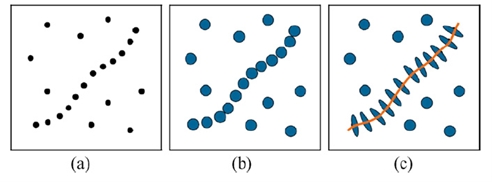
For visualization purposes the ball component represented by an ellipsoid with minor radius λ_2, and stick component is represented with its confidence factor being the major radius in the direction of the normal, and as shown in Figure 1. [2] As shown in Figure 1.c this representation shows clear distinction between the points lying on the curve compared to the outliers, which can now be interpreted by the voting method.
Figure 1: Tensor voting example: (a) input points, (b) ball tensor encoding, (c) deformation of tensors reveals the salient curve.
The voting itself also takes place on varying scales corresponding to the scales at which the pixels were selected, where each voting pixel is compared to its scale neighborhood. The output of this process is another tensor which shows an increase in the confidence factor when there is significant correspondence in the normal to the curve within the neighborhood, and decreased when the pixel has little or no correspondence with this normal. The final result of processing all of the voting pixels in this way is a matrix of matrices corresponding to each of the chosen pixels new corrected vote, which can then be used to interpolate the value of pixels between votes or register a series of images as will be discussed later. In general the premise of this original algorithm is very strong and does quite well to find underlying patterns in pixels, but does have its fair share of drawbacks.
In this original algorithm was applied once at a single scale that was chosen through trial-and-error, selecting the best resulting image, thus leading to criticism which will be presented in Section 2a. The amount of computation needed for this original method is high, and the range of resulting images produced can vary so widely with scale that the best scale factor, usually denoted as σ_s, is not always apparent. This scale factor also plays a major part in the recreation of curves, in that unless the curves are on the order of the scale, they can be misinterpreted as lines or outlying points. The algorithm works well for linear objects, but poorly reconstructs drastic changes in gradient tangents as small radius circles or spirals exhibit, which will also be shown in Section 2a.
For time lapse images, calculations based on pixel gradient become overbearing, as each processed image contains pixels that are the same frame to frame, or groups of pixels that move together across the frame. This is the main criticism that will be discussed in Section 2c, in which a new form of representation will be established that moves away from the vote representing the intensity and direction of the proposed curve, and instead becomes a representation of the direction and the magnitude of pixel velocity across the frame.
2. Improvements to Original Tensor Voting Framework:
2.a Varying Scale:
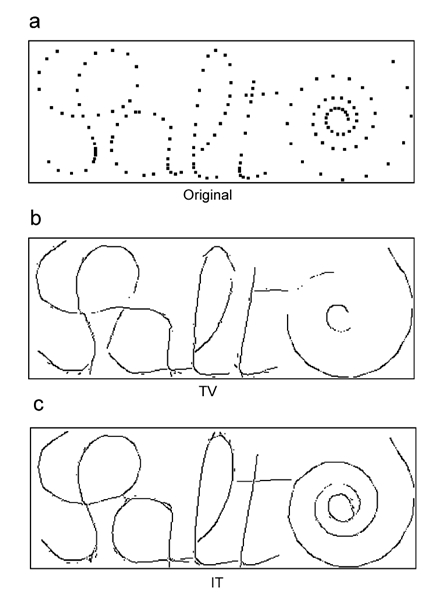
Fischer et al proposed that the method should not be done in one iteration, but multiple iterations of the voting process at varying scale from larger to smaller. This removes noise, but retains the pixels that correspond to a line of rapidly changing direction, like a spiral. This method does show notably better results than the original TV framework, as shown in Figure 2 [1], at reproducing curves. This method does come at the cost of having to iterate through the voting procedure, which as noted before is computationally heavy, but would be faster than the trial-by-error method, where the only way of determining if the σ_s was correct is to interpolate the resulting matrix and reproduce a new image.
Figure 2: Hand Drawn Example. (a) Test Image "Salt" (b) Interpolation using original TV (c) Interpolation using Iterative Tensor Method [1]
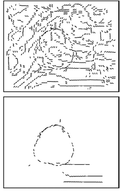
This computation method still has inherent computational inefficiencies, however, as the whole voting matrix is recalculated at every scale, where the larger scale changes are still present at the smaller scale. A new iteration algorithm starts at a large scale tensor voting, takes what it determined to be outliers, and processes those points in the next iteration at a finer scale to determine if they correspond to one another. In this method not only do fewer and fewer points have to be processed at each iteration, but the changes that they can possibly create can be approximated before processing and used as a measure as to when to stop iterating. This method will inherently perform better in high noise situations if the noise distribution is known. A plot of the distribution of the saliency of the remaining pixels is created. If it’s vastly different than the expected noise, it most likely contains many inlying pixels. This critique and approach was also put forth by Loss et al, with remarkable results, inputting very noisy images and returning almost exclusively the desired pixels as shown in Figure 3. [2]
Figure 3: Pear on wood with SNR down to 5%
2.b Losing Scale Variant Curves:
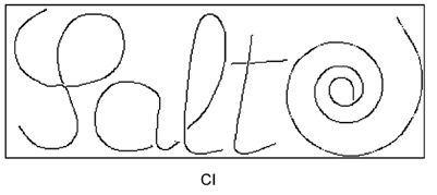
The second effect of constant scale is much more significant on curves than on straight lines, as curves outside the scale are greatly reduced in intensity and resolution, or declared as noise and completely removed, as the algorithm is looking to reduce changes in intensity gradient. By adding some measure of curvature while comparing pixels in a neighborhood, this could be compared while voting. Through much the same process drastically different curvature votes can be reduced or eliminated as they are most likely noise. As the eigenvectors of the gradient matrix are part of the input data, it isn’t much of a stretch in computation to compare them to the output matrix being created to see if they have similar proportions. This would represent that they are of the same scale curve and leaving some allowance for change, curves of varying scale as in spirals can also be retained. The application of this approach put forth by Fischer et al, also allows for an enhancement coefficient which would make the algorithm increase the votes of curves while decreasing votes for straight lines, and shows near perfect results on the example in Figure 2 as shown in Figure 4. [1] The method put forth in Fischer et al is also highly dependent upon the same iterative method they put forth as described in Section 2a, and therefore has similar inefficiencies as discussed, but also would have the same possibility for improvement through a method like the one put forward by Loss et al. However these specific articles did not explore this specific point.
Figure 4: Hand Drawn Image of 'salt' Processed by "Curve Improvement" Method [1]
2c. Inefficiencies Voting on Pixel Intensity Gradient:
It’s been established that the original voting framework has its fair share of deficiencies within the algorithm itself. Putting those points aside, it’s worthwhile to explore the idea that maybe that there are problems with the original representation when dealing with more dimensions. In the instance of time lapse photos or video, the representation of intensity gradient can be very inefficient in that most of the time the background image remains the same while objects move across the frame. In actual application in computer vision, robotics, or automation, rarely ever is a single image used, and usually some distinction between objects and the background is sought, all while requiring fast computation times to approach real time environments. As shown in previous sections, distinguishing these objects in general is possible, but with methods based upon the changes in pixel intensity over time varying images further multiplies the computation time, as each image needs to be processed over a varying scale, et cetera. The method works well, but requires a change of basis to now track pixel velocities over time through the stack of images.
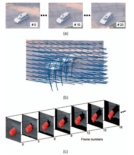
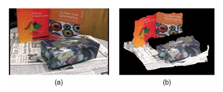
The approach taken by Min and Medioni is based upon these shortcomings where they transform the tensor 5 dimensions being space x, space y, time, velocity x, and velocity y. The input is a series of images, with the reference image taken as the image in the middle of the stack. From this reference image, intensity changes from image to image are recorded as velocities in the x and y directions of each individual pixel. From here the computation methods are very similar to TV as those pixels with similar velocities are grouped and kept, where as pixels of varying velocity are grouped separately to be thrown out or processed as another object moving in the image. This method was shown to produce favorable results with both stationary and moving cameras as the basis for comparison is the middle image in the stack, which is the time domain, and not a point in space, as shown in Figure 5. [3] Min and Medioni go on to show that similar methods can be used to reconstruct 3D images through the use of a moving camera, even if the reference objects are moving as well, based upon the same algorithm as shown in Figure 6. [3]
Figure 5: (a) Input Sequence of Images with both Car and Camera Moving (b) Overlay of Trajectories (c) Pixel Level Tracking of the Car
Figure 6: 3D Reconstruction (a) One of the Two Given Images (b) Generated 3D Construction
Concluding Remarks:
In each of the three articles the underlying theme is addressing computation time, as it is a known shortcoming of this processing technique compared to simple edge detection. Each article’s main conclusions are sound in their own right, but as time passes and new ways of thinking about this method are developed, improvements will be made, and old techniques become obsolete. As computing power has become faster and more widely available, this technique is allowing for interpretation of images by computer that used to have any significance to a human observer as well as surpassing the average ability for the human mind to register 2D images into 3D.
References:
[1] Iterated tensor voting and curvature improvement
Sylvain Fischer, Pierre Bayerl, Heiko Neumann, Rafael Redondo, Gabriel Cristobal
Signal Processing: Volume 87 Issue 11, November 2007, Pages 2503-2515
[2] An Iterative Multi-Scale Tensor Voting Scheme for Perceptual Grouping of Natural Shapes in Cluttered Backgrounds
Leandro A. Loss, George Bebis, Mircea Nicolescu and Alexei Skurikhin
Journal of Computer Vision and Image Understanding (CVIU)
[3] Inferring Segmented Dense Motion Layers Using 5D Tensor Voting
Changki Min and Gerard Medioni
IEE Transactions on Pattern Analysis and Machine Intelligence, VOL. 30, NO. 9, SEPTEMBER 2008 pages 1589-1620
I have been working with two different resources for developing tensor voting framework:
1: code developed in VXL by Brad King
2: code developed in Matlab by Trevor Linton
Obtaining and building the VXL version:
1) Download an SVN tool ->([1])
2) Use the SVN tool to download https://vxl.svn.sourceforge.net/svnroot/vxl/trunk
a) For tortoisesvn go to desired file location, right click, SVN checkout, put in the URL above and give desired file location and allow to download (internet access needed)
3) Download and install CMake version 2.6 or greater from ->[2]
4) Start Cmake
a) Put the root folder location downloaded from the svn as source code
b) Create a file on the same level as the root folder and call it *_bin for the binary builds
c) Make sure the following options are configured (must be set to advanced view near search)
BUILD_CONTRIB
BUILD_CORE_GEOMETRY
BUILD_CORE_IMAGING
BUILD_CORE_NUMERICS
BUILD_CORE_SERIALISATION
BUILD_CORE_UTILITIES
BUILD_EXAMPLES
BUILD_MUL
BUILD_RPL
BUILD_RPL_RGTL
BUILD_RPL_RTVL *** appears after first configure completes
BUILD_VGUI
d) After first click of configure, the checking of BUILD_RPL_RTVL, click generate and select the desired c++ compiler
From here you should now have the correct VXL libraries for Brad's TVF, I recommend checking out "rtvl_hello" as this is a primary introduction into how to run the function calls necessary for 2D voting
Obtaining and building the Matlab version:
1) Obtain the TVF library from Matlab Central -> [3]
2) Unzip the file and add it to the file path in matlab
This should be all you need to run the TVF libraries in Matlab
About the Code
Brad's code:
This code was written in VXL after his doctoral thesis work on Range Data Analysis by Free Space Modeling and Tensor Voting, and the code is now publicly available. This includes the ability to vote on both 2D and 3D data sets (distinguished by the 2 or 3 in the function name).
My only true critique of this code is the VXL libraries are poorly documented, thus making the analysis and use of the code a very steep learning curve for those not familiar with the VXL libraries. His code, again, has the ability to run both 2D and 3D data-sets which allows for great versatility, especially in the area of multi-dimensional microscopy. As the voting takes place cumulatively, one can also adapt the code to do multi-scale voting to provide better reconstruction. It isn't set up in such a way that would allow for efficient multi-scale voting based upon scale saliency as described by L. Loss et al., An iterative multi-scale tensor voting scheme for perceptual grouping ..., Comput. Vis. Image Understand. (2008), doi:10.1016/j.cviu.2008.07.011, but will still accomplish the same goal.
As I haven't had much experience with VXL, I created Matlab code to create a data set that included voting pixel location and vote direction into a text file with the file extension of .BKI. Within the VXL code I read in the data from this text file, go through the voting process, and output the pixel location and its saliency map values, into another text file "voting_output.txt". I then created Matlab code that then reads in this data and reconstructs the saliency map, and generates the best fit line through the saliency map.
rtvl_hello (adapted)
/* Copyright 2010 Brad King
Distributed under the Boost Software License, Version 1.0.
(See accompanying file rtvl_license_1_0.txt or copy at
http://www.boost.org/LICENSE_1_0.txt) */
/* Adapted by Sam Gilbert to take text file input with
created .BKI extension, coded for multi–scale, and to
create an output file with the saliency map*/
#include <rtvl/rtvl_tensor.hxx>
#include <rtvl/rtvl_vote.hxx>
#include <rtvl/rtvl_votee.hxx>
#include <rtvl/rtvl_voter.hxx>
#include <rtvl/rtvl_weight_smooth.hxx>
#include <vnl/vnl_vector_fixed.h>
#include <vnl/vnl_matrix_fixed.h>
#include <vcl_vector.h>
#include <vcl_iostream.h>
int main()
{
int Data_PTS = 0;
int loc_x = 0;
int loc_y = 0;
int x_dim = 0;
int y_dim = 0;
float T11 = 0;
float T12 = 0;
float T21 = 0;
float T22 = 0;
vcl_vector< vnl_matrix_fixed<double, 2,2> > votee_matrices(0.0);
vnl_matrix_fixed<double,2,2> zero_matrix;
zero_matrix(0,0) = zero_matrix(1,0) = zero_matrix(0,1) = zero_matrix(1,1) = 0;
vcl_vector< vnl_vector_fixed<double, 2> > inlocations (0.0);
vcl_vector< vnl_vector_fixed<double, 4> > Tensors (0.0);
vcl_vector< vnl_vector_fixed<double, 2> > outlocations(0.0);
vnl_vector_fixed<double,2> zero_location(0.0);
vnl_vector_fixed<double,4> zero_location_4(0.0);
// IN file location <-- !!! Change to your own location !!!
FILE *fp1 = fopen("C:\\YOUR INPUT FILE NAME EXTENSION GOES HERE","r");
rewind (fp1);
fscanf(fp1,"%d %d %d\n",&Data_PTS, &x_dim, &y_dim);
vcl_cout << "Number of Voting points = " << Data_PTS << vcl_endl;
for(int counter = 0; counter <= Data_PTS; counter++)
{
fscanf(fp1, "%d %d %f %f %f %f\n", &loc_x, &loc_y, &T11, &T12, &T21, &T22);
inlocations.push_back(zero_location);
inlocations[counter][0] = loc_x;
inlocations[counter][1] = loc_y;
Tensors.push_back(zero_location_4);
Tensors[counter][0] = T11;
Tensors[counter][1] = T12;
Tensors[counter][2] = T21;
Tensors[counter][3] = T22;
}
fclose(fp1);
int counter = 0;
for(int counterx = 0; counterx <= x_dim; counterx++)
{
for(int countery = 0; countery <= y_dim; countery++)
{
votee_matrices.push_back(zero_matrix);
outlocations.push_back(zero_location);
outlocations[counter][0] = counterx;
outlocations[counter][1] = countery;
counter++;
}
}
vnl_matrix_fixed<double, 2, 2> voter_matrix (0.0);
// Out file location --> !!! Change to your own location !!! <---
FILE *fp = fopen("C:\\YOUR OUTPUT FILE EXTENSION GOES HERE","w");
vcl_cout << "Voting, Please wait..." << vcl_endl;
for(int Scale_counter = 2; Scale_counter < 3; Scale_counter++) // ENTER IN UPPER AND LOWER SCALE LIMITS HERE
{
rtvl_weight_smooth<2> tvw(Scale_counter);
for( int counter = 0; counter< inlocations.size() ; counter++)
{
voter_matrix(0,0) = Tensors[counter][0];
voter_matrix(1,0) = Tensors[counter][2];
voter_matrix(0,1) = Tensors[counter][1];
voter_matrix(1,1) = Tensors[counter][3];
rtvl_tensor<2> voter_tensor(voter_matrix);
rtvl_voter<2> voter(inlocations[counter], voter_tensor);
for(int vcounter = 0; vcounter< outlocations.size(); vcounter++)
{
// Use "rtvl_votee" to encapsulate a site (location + output tensor).
rtvl_votee<2> votee(outlocations[vcounter], votee_matrices[vcounter]);
// Compute one vote.
rtvl_vote(voter, votee, tvw);
}
// Decompose the result.
}
}
for(int counter = 0; counter< outlocations.size() ; counter++)
{
rtvl_tensor<2> votee_tensor(votee_matrices[counter]);
vnl_vector_fixed <double,2> base = votee_tensor.basis(0);
vnl_vector_fixed <double,2> base2 = votee_tensor.basis(1);
fprintf(fp,"%0.3f %0.3f %0.3f %0.3f %0.3f %0.3f\n",outlocations[counter][0],outlocations[counter][1],base[0],base[1],base2[0],base2[1]);
}
fclose(fp);
return 0;
}
Brad_King_In (Matlab file to create input files for rtvl)
% function Brad_in(file_name)
% This function takes standard image files and creates .BKI file for use
% with Brad King's code in VXL ** NOTE: Canny filter is used for
% preliminary edge detection to reduce number of votes which improves
% results on noisy grayscale images
file_name = 'YOUR FILE NAME HERE';
%%%%%%%%%%%%% The main.m file %%%%%%%%%%%%%%%
% The algorithm parameters:
% 1. Parameters of gradient direction filters - region used in the gaussian
% edge detection to determine the direction of the vote
% X-axis direction filter:
%% SCALE of gradient direction in x = Nx1, Nx2
Nx1=3;Sigmax1=1;Nx2=3;Sigmax2=1;Theta1=pi/2;
% Y-axis direction filter:
%% SCALE of gradient direction in y = Ny1, Ny2
Ny1=3;Sigmay1=1;Ny2=3;Sigmay2=1;Theta2=0;
% Get the initial image
[w]=imread(file_name);
[w,thresh] = edge(w,'canny');
w = double(w);
% X-axis direction edge detection
filterx=d2dgauss(Nx1,Sigmax1,Nx2,Sigmax2,Theta1);
Ix= conv2(w,filterx,'same');
% Y-axis direction edge detection
filtery=d2dgauss(Ny1,Sigmay1,Ny2,Sigmay2,Theta2);
Iy=conv2(w,filtery,'same');
[m2,n2] = size(Ix);
dot_edge_file = [0 0 0 0 0 0];
for i=2:m2-1 %% ignore edge pixels
for j=2:n2-1 %% ignore edge pixels
if abs(Ix(i,j))> 0 || abs(Iy(i,j))> 0 %% ignore pixels with no gradient
%% get tensor votes from intensity gradients
K11 = Ix(i,j)^2;
K12 = Ix(i,j)*Iy(i,j);
K21 = Ix(i,j)*Iy(i,j);
K22 = Iy(i,j)^2;
% trace/2
t = (K11+K22)/2;
a = K11 - t;
b = K12;
ab2 = sqrt(a.^2+b.^2);
theta = atan2( ab2-a, b );
dot_edge_file = [dot_edge_file; i j cos(theta) sin(theta) -sin(theta) cos(theta)];
end
end
end
[m,n] = size(Ix);
dot_edge_file = dot_edge_file(2:length(dot_edge_file),:);
loc_x = dot_edge_file(:,1);
loc_y = dot_edge_file(:,2);
T11 = dot_edge_file(:,4);
T12 = dot_edge_file(:,3);
T21 = dot_edge_file(:,6);
T22 = dot_edge_file(:,5);
fid = fopen([file_name(1:length(file_name)-3),'BKI'], 'wt');
fprintf(fid, '%.0f %.0f %.0f\n', length(dot_edge_file), m, n);
%% first line in output file is:
% #of votes y-dimension x-dimension
%% **dimensions of original image
for i = 1:length(loc_x)
fprintf(fid, '%.0f % .0f % .4f % .4f % .4f % .4f\n', loc_x(i), loc_y(i), T11(i), T12(i), T21(i), T22(i));
end
%% each line thereafter is:
%% x-location y-location T11 T12 T21 T22
%% where T11 is top left, T12 is top right, T21 bottom left, T22 bottom
%% right of the tensor matrix
fclose(fid);
Brad_King_Out (Matlab file to reconstruct the output from rtvl)
%% rough reconstruction of saliency map output from Brad King's rtvl
A = dlmread('voting_output.txt');
[m2,n2] = size(A);
%% reconstruct tensors from the saliency map
K11 = A(:,3);
K12 = A(:,4);
K21 = A(:,5);
K22 = A(:,6);
[n,p] = size(K11);
o1 = zeros(n,p,2);
o2 = zeros(n,p,2);
o3 = zeros(n,p);
o4 = zeros(n,p);
% trace/2
t = (K11+K22)/2;
a = K11 - t;
b = K12;
ab2 = sqrt(a.^2+b.^2);
o3 = ab2 + t;
o4 = -ab2 + t;
theta = atan2( ab2-a, b );
o1(:,:,1) = cos(theta);
o1(:,:,2) = sin(theta);
o2(:,:,1) = -sin(theta);
o2(:,:,2) = cos(theta);
e1 = o1;
e2 = o2;
l1 = o3;
l2 = o4;
z = l1-l2;
l1(z<0.4) = 0;
l2(z<0.4) = 0;
r = 30; %% Outer scale - scale for best fit lines through the image
epsilon = pi/4; %% radians of search for strongest saliency from the
%% reconstructed point's tensor direction
q = l1-l2; % subtraction of the two eigan values
[h w] = size(l1); % getting the size of the image
re = zeros(h,w,'double'); %intializing the output matrix
%% generate the best fit line throught the tensor matrix
[X,Y] = meshgrid(-r:1:r,-r:1:r);
t = atan2(Y,X);
l = sqrt(X.^2 + Y.^2);
q1 = zeros(2*r+h, 2*r+w);
q1((r+1):(h+r), (r+1):(w+r)) = q;
D = find(q1>0);
[h w] = size(q1);
for i=1:size(D,1)
[y,x] = ind2sub(h, D(i));
X2 = l.*cos(t + atan2(e1(y-r,x-r,2),e1(y-r,x-r,1)));
Y2 = l.*sin(t + atan2(e1(y-r,x-r,2),e1(y-r,x-r,1)));
t2 = abs(atan2(Y2,X2));
t2(t2 > pi/2) = pi - t2(t2 > pi/2);
t2(t2 <= epsilon) = 1;
t2(t2 ~= 1) = 0;
t2(l > r) = 0;
z = q1((y-r):(y+r),(x-r):(x+r)).*t2;
z = max(z > q1(y,x));
if max(z(:)) == 0
re(y-r,x-r) = 1;
end
end
img = zeros(max(A(:,2))+1,max(A(:,1))+1);
for i = 1:length(A)
img(A(i,2)+1,A(i,1)+1) = re(i);
end
img = flipud(img)
figure, imshow(img);
Matlab Code:
An implementation of Medioni's Tensor Voting, publicly available on Matlab Central. This code was developed to only process 2D images based upon ".edge" files included in the package. The code is also capable of running at multi-scale, but again is just done through a simple iterative adding rather than as described by Loss et al.
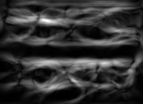
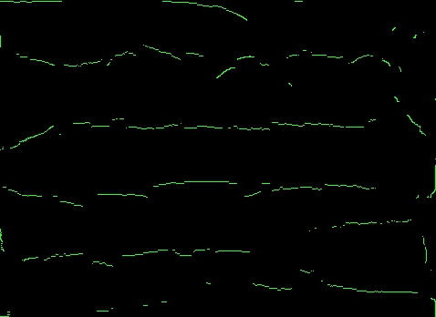
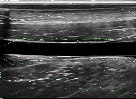
My critiques of this code is that not only is code that produced these ".edge" files not provided, but there is no documentation as to what information is in the file. I've guessed that the data is related to pixel location and gradient direction, and have created code that allows for the creation of the files from ordinary 2D gray-scale images, and it seems to be correct. If processing grayscale images with wide varying noise, such as ultrasound images, I would recommend canny edge detection to reduce the number of voting pixels to both improve computation time and saliency results, as too many conflicting votes can diminish the desired votes.
Create_dot_edge (creates .edge file used by the Matlab TVF)
% function create_dot_edge(file_name)
% This function takes standard image files and creates .edge file for use
% with the tensor voting framework (see TVF\demo). ** NOTE: this uses the
% canny filter to reduce the number of input pixels
file_name = 'YOUR FILE EXTENSION GOES HERE';
%%%%%%%%%%%%% The main.m file %%%%%%%%%%%%%%%
% The algorithm parameters:
%1. Parameters of gradient direction filters - region used in the gaussian
% edge detection to determine the direction of the vote
% X-axis direction filter:
%% SCALE of gradient direction in x = Nx1, Nx2
Nx1=3;Sigmax1=1;Nx2=3;Sigmax2=1;Theta1=pi/2;
% Y-axis direction filter:
%% SCALE of gradient direction in y = Ny1, Ny2
Ny1=3;Sigmay1=1;Ny2=3;Sigmay2=1;Theta2=0;
% Get the initial image
[w]=imread(file_name);
figure(1);colormap(gray);
imagesc(200,200,w);
title(['Image: ', file_name]);
[w,thresh] = edge(w,'canny');
w = double(w);
figure; imshow(w)
% X-axis direction edge detection
filterx=d2dgauss(Nx1,Sigmax1,Nx2,Sigmax2,Theta1);
Ix= conv2(w,filterx,'same');
% Y-axis direction edge detection
filtery=d2dgauss(Ny1,Sigmay1,Ny2,Sigmay2,Theta2);
Iy=conv2(w,filtery,'same');
[m,n] = size(Ix);
gradient_directions = zeros(m,n);
dot_edge_file = [0 0 0];
for i=1:m
for j=1:n
if Ix(i,j)<0&& Iy(i,j)<0
gradient_directions(i,j) = rad2deg(3*pi/2 -(atan(Iy(i,j)/Ix(i,j))));
dot_edge_file = [dot_edge_file; i j gradient_directions(i,j)];
else if Ix(i,j)>0&& Iy(i,j)<0
gradient_directions(i,j) = rad2deg(3*pi/2 + (atan(Iy(i,j)/Ix(i,j))));
dot_edge_file = [dot_edge_file; i j gradient_directions(i,j)];
else if Ix(i,j)<0&& Iy(i,j)>0
gradient_directions(i,j) = rad2deg(pi/2 - (atan(Iy(i,j)/Ix(i,j))));
dot_edge_file = [dot_edge_file; i j gradient_directions(i,j)];
else if Ix(i,j)>0&& Iy(i,j)>0
gradient_directions(i,j) = rad2deg(pi/2 -(atan(Iy(i,j)/Ix(i,j))));
dot_edge_file = [dot_edge_file; i j gradient_directions(i,j)];
end
end
end
end
end
end
dot_edge_file = dot_edge_file(2:length(dot_edge_file),:);
loc_x = dot_edge_file(:,1);
loc_y = dot_edge_file(:,2);
ang = dot_edge_file(:,3);
fid = fopen([file_name(1:length(file_name)-3),'edge'], 'wt');
fprintf(fid, '%.f\n', length(dot_edge_file)); %% first line is the number
%% of votes generated
for i = 1:length(loc_x)
fprintf(fid, '%.0f % .0f % .4f\n', loc_x(i), loc_y(i), ang(i));
end
%% subsequent lines are x-location, y-location and the angular direction
%% of the normal in degrees
%% output file name is the same as the input file name with the file
%% extension .edge
fclose(fid);
demo (processes the .edge file with the TVF and reconstructs the best fit line through the saliency map)
%%function demo(file)
%% This file calls the functions that make up the TVF in matlab, input is a .edge file, output is the best fit reconstruction
file = 'YOUR FILE EXTENSION HERE.edge';
im = im2double(imread('YOUR IMAGE FILE EXTENSION HERE.TIF/JPG/etc'));
% Read in the dot edge file and turn it into a bitmask image
T = read_dot_edge_file(file);
[e1,e2,l1,l2] = convert_tensor_ev(T);
figure, imshow(l1);
% Run the tensor voting framework
T = find_features(l1,25);
T2 = find_features(l1,35);
T3 = find_features(l1,45);
T = T+T2+T3;
%% multi-scale implementation- second parameter of find_features
%% is the scale factor
% Threshold unimportant data that may create noise in the
% output.
[e1,e2,l1,l2] = convert_tensor_ev(T);
z = l1-l2;
l1(z<0.3) = 0;
l2(z<0.3) = 0;
%% zeros votes of low saliency
T = convert_tensor_ev(e1,e2,l1,l2);
figure,imshow(l1-l2,'DisplayRange',[min(z(:)),max(z(:))]);
% Run a local maxima algorithm on it to extract curves
re = calc_ortho_extreme(T,25,pi/8);
% second parameter of calc_ortho_extreme is reconstruction scale factor,
% third parameter is the range of angles (with respect to the curent tensor angle
% in which it looks to reconstruct
%figure, imshow(re);
figure
[m,n] = size(re);
im2 = im(1:m,1:n) + flipud(re);
imshow(im2)
%% this shows the reconstruction super-imposed upon the original image
end
Results
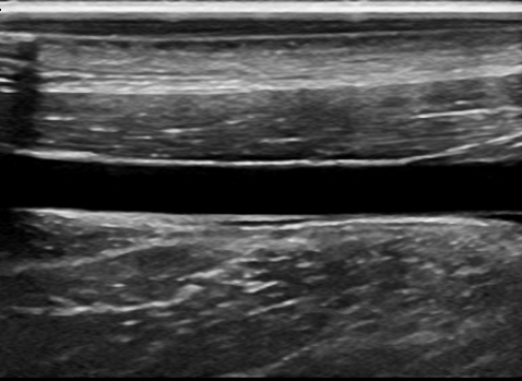
Input image
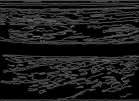
Output from Canny edge detect
Output saliency map from Matlab TVF
Best fit Reconstruction from Matlab TVF
Overlay of reconstruction and original image
