Histopathology
(→Computing Associations) |
(→Training and Classification) |
||
| Line 81: | Line 81: | ||
===Training and Classification=== | ===Training and Classification=== | ||
| + | For [[NucleusEditor#KPLS_Classifier|training and classification]] see the eponymous section in the [[NucleusEditor#KPLS_Classifier|nucleus editor]] page | ||
==Histopathology Program in the IDL environment== | ==Histopathology Program in the IDL environment== | ||
Revision as of 23:01, 8 February 2010
This page describes the FARSIGHT approach applied to digital histopathology. In current clinical practice, histological specimens (from biopsy) are stained using traditional stains like hematoxylin and eosin, and inspected under a standard brightfield microscope. The scoring of histopathology slides is currently very qualitative and approximate. Our goal is to enable objective and quantitative scoring of slides with a particular emphasis on quantifying the distribution of molecular biomarkers that indicate specific disease conditions. For example, estrogen receptor (ER), progesterone receptor (PR), and Ki67 are examples of molecular biomarkers that are important for diagnosing and sub-typing breast cancers. Our method is based on three basic principles: (i) delineate each cell in the image field as accurately as possible; (ii) identify the types of all cells in the field; and (iii) quantify biomarkers on a cell-by-cell basis in a selective manner based on cell type.
In this application, the images are spatially two-dimensional, but much richer in terms of spectral data per pixel. The specimens are multiplex immunolabeled to highlight key tissue structures of interest (cell nuclei, membranes, cytoplasmic regions of certain cell types, etc.), and the molecular biomarkers of interest. These immunolabeled specimens are subjected to multi-spectral microscopy. The spectral cubes are computationally unmixed to produce a set of non-overlapping channels that are analyzed using the FARSIGHT divide & conquer associative image analysis strategy.
Currently, this system is implemented using a combination of C++ and IDL. It is currently being translated to a C++ and Python based system. The illustrations and instructions below refer to the IDL/C++ system. Users need to download and install the free IDL virtual machine from ITT. This page does require you to register.
Contents |
Background and motivation
Detecting molecules of interest and quantifying them plays an increasingly important role in modern medical diagnosis and treatment planning[1]. Currently, most systems are visually based qualitative descriptors which suffer from the consequent limitations. There are other algorithms that quantify biomarkers on a pixel-by-pixel basis or a regional basis[2-5]. Segmenting the cells and nuclei allows us to classify the different cell types based on antigens that mark specific cell. This enables us to quantify the biomarker of interest in the relevant cell type. This is a more biologically relevant measure and can be more useful in medical diagnosis.
Histopathology Program in c++
The histopathology tool in Farsight inherits all the GUI capabilities of the Nucleus Editor and extends the functionality for use in cytometric analysis of histopathology samples. For efficient editing of nuclear segmentation and to use all the functional capabilities of the GUI, read the Nucleus Editor page and then proceed with this page. The work-flow for the cytometric quantification of biomarkers and classification of cells is divided into five steps.
- Load and pre-process channels
- Nucleus Segmentation
- Whole Cell Segmentation
- Computing Associations
- Training and Classification
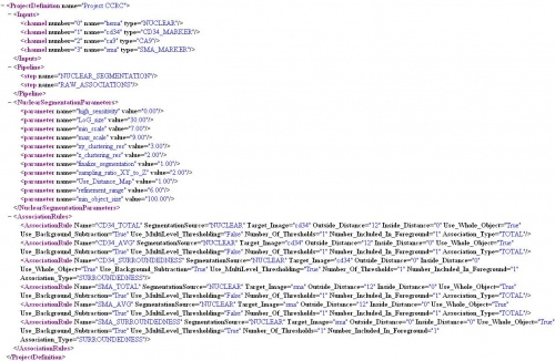
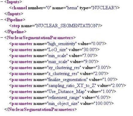
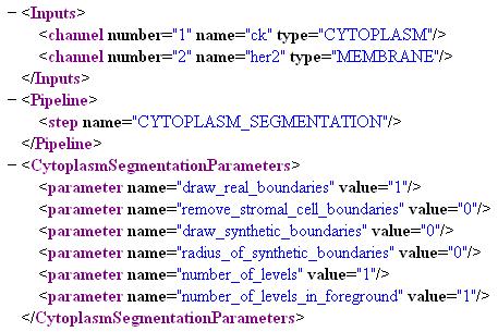
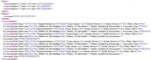
These steps are to be specified in a "Project definition" file that holds all the steps that are necessary to process similar sets of images. The purpose of this to enable batch processing of large sets of images. A sample Project definition file is shown below. First, the input images are specified with their respective names and tags. Second, the steps in the Pipeline are defined. As of now, only NUCLEAR_SEGMENTATION, CYTOPLASM_SEGMENTATION and RAW_ASSOCIATIONS steps can be pipe lined. Methods CLASSIFY and ANALYTE_MEASUREMENTS will be added soon. Third, nucleus segmentation parameters are specified. Fourth, the whole cell segmentation parameters and the fifth set is the associations. A typical project definition file is shown below.
Load and pre-process channels
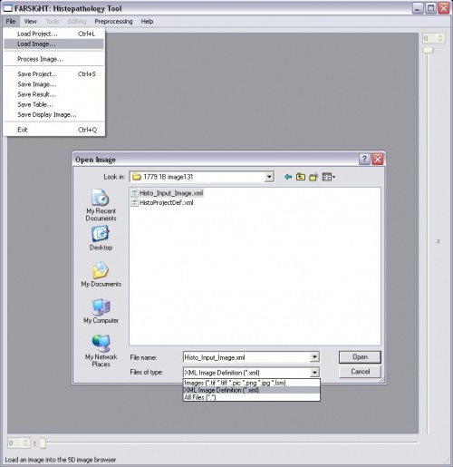
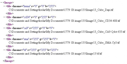
Images can be loaded as is from the hard disk. The supported file formats have the following extensions .tif, .pic, .png, .jpg and .lsm Since there is no open source format with an accompanying tool with which a user can conveniently synthesize images composed of channels multiple channels and append meta-data, the histopathology tool includes a method to load channels and meta-data specified in a xml file. The full path of each image has to be specified here. The display color-space to which the image is rescaled is specified as <r="___" g="___" b="___"> along with the channel name. The rage for each color is between 0 and 255. If r=g=b=255 the image will be loaded with its native color range but such images can not be used in any processing step. The conversion and rescaling of RGB images loaded as single channels is done internally, so, the format of the image is not a factor. The tag <chname="___"> specifies the channel name which is used to identify the channel in the processing step. Caution: The case of channel name strings have to match in both the image file and the project definition file.
 -Click "File->Load Image"
 -Choose either a single image of type .tif, .pic, .png, .jpg, .lsm or multiple images specified in an .xml file
 -Click "Open" to load the image
 -To pre-process a channel, click Processing and then choose a filter
Nucleus Segmentation
To enable this step, add the step "NUCLEAR_SEGMENTATION" to the pipeline and this is performed on the first channel that has the type tag "NUCLEAR". The parameters are described in detail on the Nucleus Segmentation page.
 -Use the tag "NUCLEAR" for the channel stained for nuclei
 -Add the step "NUCLEAR_SEGMENTATION" to the pipeline
 -Either add the nucleus segmentation parameters or skip to use the defaults
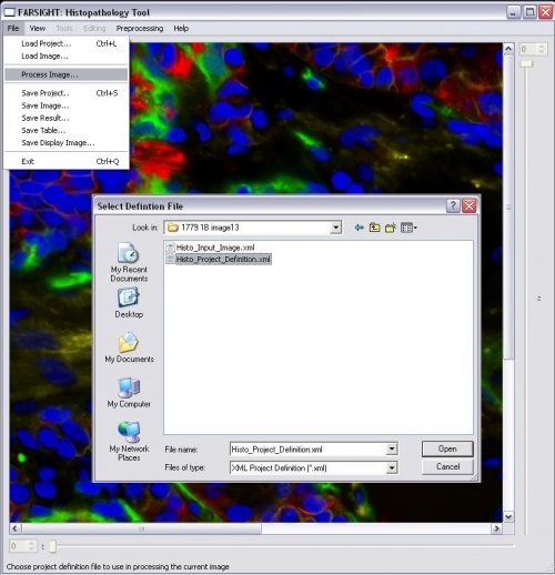
 -Click File->Process Image and select the project definition file to start processing
 -After initial processing, there will be a pause to allow the user to edit the nucleus segmentation result
 -Click on the green "proceed" arrow to continue with the pipeline after editing the nucleus segmentation
Whole Cell Segmentation
To enable this step, add the step "CYTOPLASM_SEGMENTATION" to the pipeline and this is performed on the first channel that has the type tag "CYTOPLASM". Use the tag "MEMBRANE" if there is a channel with the membrane labeled and the gradients from this channel are to be used to Define the cell boundaries. The parameters are(the first three are binary, i.e., '1' or '0'):
1. draw_real_boundaries: Use image cues to draw cell boundaries
2. remove_stromal_cell_boundaries: Remove cell boundaries from cells that have no extra-nuclear domains
3. draw_synthetic_boundaries: Generate geometric domains for cells with no extra-nuclear domains if above two parameters are set to '1', if the first parameter is set to '0' then the cell domains for the entire slide are generated geometrically
4. radius_of_synthetic_boundaries: This is set maximum distance of the geometric cell boundary from the boundary of the nucleus
5. number_of_levels: Number of thresholds used in generating the binary
6. number_of_levels_in_foreground: Number of levels from above included in the foreground while generating the binary
 In the project definition file:
-Tag the cytoplasm stained channel with "CYTOPLASM" and the membrane channel with "MEMBRANE"
-Add "CYTOPLASM_SEGMENTATION" to the pipeline
-Set the parameters
Computing Associations
The associative features code extends the object level association class to include four new parameters for background subtraction which are self explanatory and also a new type of measure called the "SURROUNDEDNESS" measure. A sample associations file is shown below
-Include the step "RAW_ASSOCIATIONS" in the pipeline
-Add association rules
Training and Classification
For training and classification see the eponymous section in the nucleus editor page
Histopathology Program in the IDL environment
The algorithms have been implemented with a custom GUI built on IDL and c++. To run the program, you will need the IDL virtual machine which is available online for free[[1]]. Soon, the GUI code will use the QT & VTK Development Framework and added to the Farsight repository.
Steps for analyzing 2-D multi-spectral images of Hisopathology samples
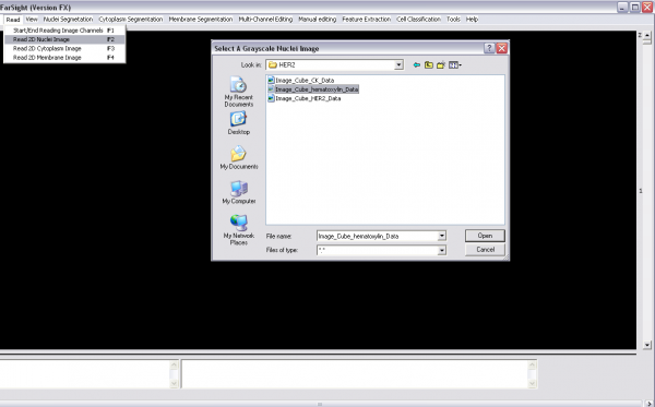
1- Read image channels one-by-one (Read menu):
  -Choose "start/end read image channels"
  -start reading the channels one by one (nuclei, cytoplasm and/or membrane channels)
  -Choose "start/end read image channels" again
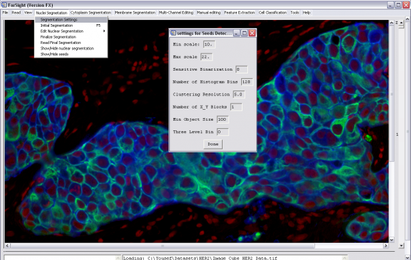
2- Start nuclear segmentation (nuclear segmentation menu):
  -Change the nuclear segmentation settings (if needed)
  -Run initial segmentation
  -Edit the nuclear segmentation results (optional). This includes merging, splitting, and deleting nuclei
  -Finalize segmentation. The segmentation result will be displayed and will be saved into a file as well
  -If a nuclear segmentation results file is already available, choose "Read Final Segmentation"
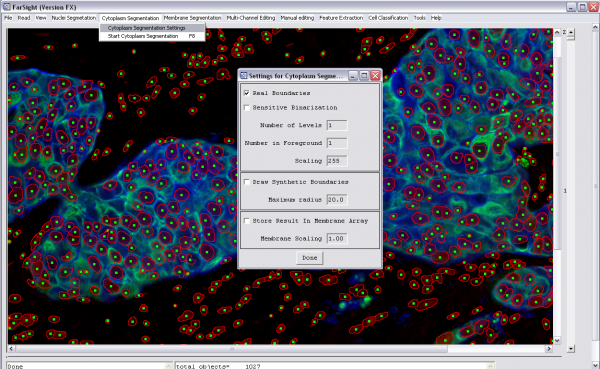
3- Start cytoplasm (or membrane) segmentation (cytoplasm segmentation menu):
  -Change the cytoplasm segmentation settings (if needed)
  -Run cytoplasm segmentation
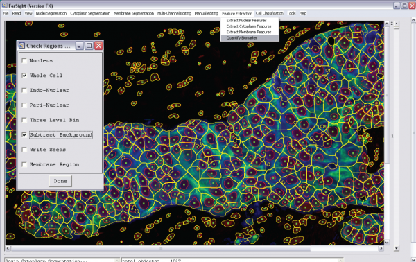
4- Quantify the biomarker (feature extraction menu):
  -Choose "Quantify Biomarker"
  -A new window will then allow you to brows for the biomarker channel (image)
  -Set the quantification options:
      -Define the region of interest
      -Choose whether or not you need to do background subtraction (two- or three-level)
  -Quantification results will be saved into a csv file
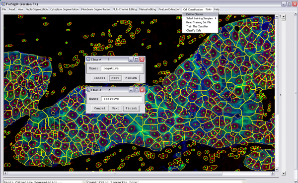
3- Classify cells (cell classification menu):
  -Define classes
  -Select training samples manually or read them from a file that was saved after previous manual selection of training samples
  -Train the classifier
  -Classify the cells
  -classification results will be displayed (by changing the seeds colors) and will be also saved into a csv file
References
- Hammerschmied CG, Walter B, Hartmann A. [Renal cell carcinoma 2008 : Histopathology, molecular genetics and new therapeutic options.]. Pathologe 2008;29(5):354-63.}
- Camp RL, Chung GG, Rimm DL. Automated subcellular localization and quantification of protein expression in tissue microarrays. Nat Med 2002;8(11):1323-7.
- Mulrane L, Rexhepaj E, Penney S, Callanan JJ, Gallagher WM. Automated image analysis in histopathology: a valuable tool in medical diagnostics. Expert Rev Mol Diagn 2008;8(6):707-25.
- Taylor CR, Levenson RM. Quantification of immunohistochemistry--issues concerning methods, utility and semiquantitative assessment II. Histopathology 2006;49(4):411-24.
- Tamai S. Expert systems and automatic diagnostic systems in histopathology--a review. Rinsho Byori 1999;47(2):126-31.
- Al-Kofahi Y, Lassoued W, Lee W, Roysam B. Improved Automatic Detection & Segmentation of Cell Nuclei in Histopathology Images. IEEE Trans Biomed Eng 2009 (in review)
- Beare R., Lehmann G. The watershed transform in ITK - discussion and new developments. The Insight Journal - 2006 January - June [[2]]
- Nath SK, Palaniappan K, Bunyak F. Accurate Spatial Neighborhood Relationships for Arbitrarily-shaped Objects using Hamilton-Jacobi GVD. Lect Notes Comput Sci 2007;4522 LNCS:421-431.
